Bloch Equation Simulation
Click for Updates!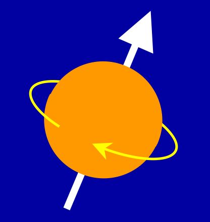
Bloch Equation SimulationClick for Updates! |
|
You will learn by far the most by doing the exercises, even though most solutions are provided. The exercises are divided into sections with the hope that you can get trhough a whole section (ie B-2) in one sitting. Since you will be writing many Matlab functions, take a little time to try varying parameters to the functions.
Lastly, development of this page is purely motivated by my desire to help to teach these concepts. Thus, your feedback is very useful to me! Please send any comments, suggestions or improved solutions, please send them to Brian Hargreaves I will put new exercises (without complete solutions) in red text. Future topics/exercises will be in orange text. Comments on any of these are welcome too!
|
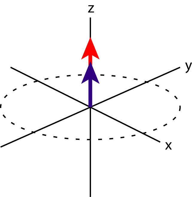
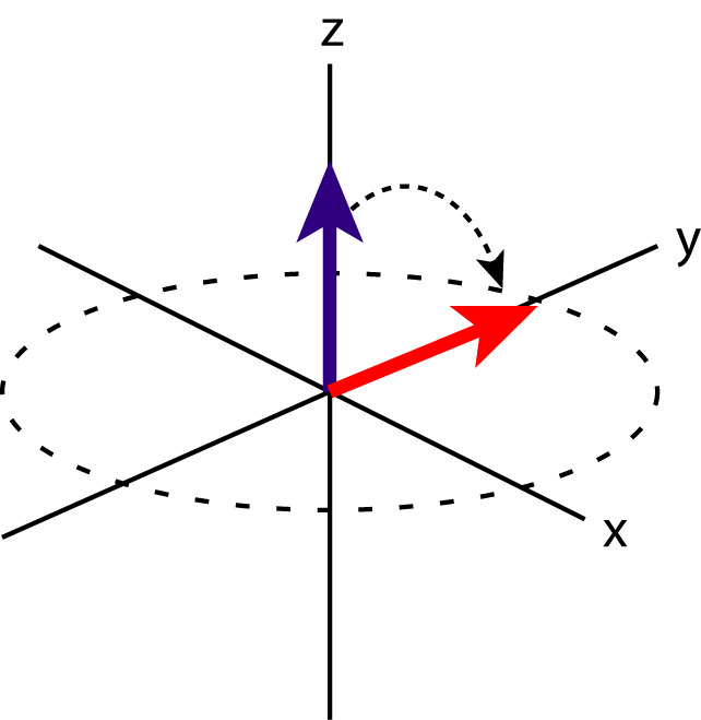
Transverse relaxation is an exponential decay
process of the x and y components of magnetization
that is always happening. Mathematically this means
Mx(t)=Mx(0)exp(-t/T2) and My(t)=My(0)exp(-t/T2). A-2a) Assume M consists of only an x component. Let's say that T2=100 ms. Ignoring other effects, what is the magnetization vector due to T2-decay after 50 ms? We'll call this magnetization M1. Answer: M1=[0.61, 0, 0]'. (still is directed along x).
Answer: A=[exp(-50/100) 0, 0;0, exp(-50/100), 0; 0, 0, 1]. |
Transverse relaxation causes shortening of the transverse component of magnetization (from blue to red), at an exponential rate with time-constant T2. |
|
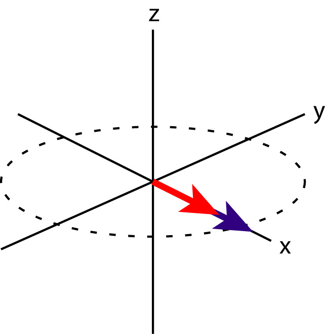
Longitudinal (z) relaxation
is a bit more complicated than transverse relaxation.
The magnetization recovers exponentially with a time constant T1,
to a non-zero value, often called M0.
Mathematically, we write Mz(t)=M0+[Mz(0)-M0]exp(-t/T1) . Note that in most of this tutorial, we just calculate all magnetization and signal levels as fractions of M0, so we assume that M0=1. A-3a) In A-2, we neglected T1-relaxation. T1-relaxation is a bit more difficult, because it is non-linear. However, you should be able to express T1-relaxation in a nice matrix form as M1=A*M+B as before, but with the addition of the 3x1 vector B. Now neglect T2-relaxation and assume that T1=600 ms, and again assume 50 ms of decay. What are A and B, if M0=1? Answer: A=[1, 0, 0;0, 1, 0; 0, 0, exp(-50/600)], B=[0, 0, 1-exp(-50/600)]'.
Answer: A=[exp(-50/100), 0, 0;0, exp(-50/100), 0; 0, 0, exp(-50/600)], B=[0, 0, 1-exp(-50/600)]'.
|
Longitudinal relaxation causes recovery of the longitudinal (z) component of magnetization (from blue to red) toward M0, at an exponential rate with time-constant T1. |
|
A-4a) Now we want to simulate precession. Precession is a rotation
about the z axis. With matrices, we can express this in the form
M1=Rz*M, where Rz is a 3x3 matrix. What is Rz if we want to rotate
by an angle phi?
Answer: Rz=[cos(phi) -sin(phi) 0;sin(phi) cos(phi) 0;0, 0, 1].
Answer: zrot.m
Answer: Rth=[0.9268 0.1268 0.3536; 0.1268 0.7803 -0.6124; -0.3536 0.6124 0.7071]. throt.m
|
Precession is a simple rotation of the magnetization vector about the longitudinal (z) axis.
|
|
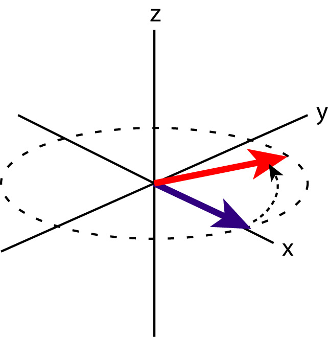
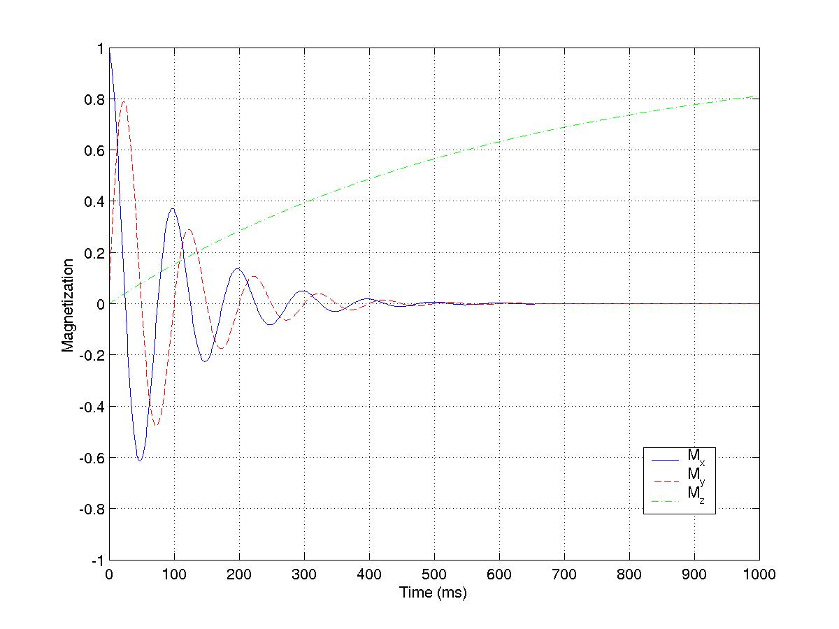
If you are new to MRI, the diagram below shows the path of transverse
magnetization as it precesses and relaxes. Click on the diagram to
the right to view an animation of the effect. A-5a) We leave excitation for a moment. Look at the matrix A for relaxation (T1 and T2 combined) and for precession, Rz. Note that they commute -- A*Rz = Rz*A. Over some interval, the effects of precession and relaxation can be applied in any order. Write a matlab function with the syntax function [Afp,Bfp]=freeprecess(T,T1,T2,df) that returns the matrices such that M1=Afp*M+Bfp. Here T is the duration of the free precession (ms), T1 and T2 are the relaxation times (ms) and df is the off-resonance frequency (Hz).
|
|
Answer: matlab code | view plot | freeprecess.m
The solutions to the Bloch Equation are three independent dynamics: T1-relaxation, T2-relaxation, and precession. Precession and T2-relaxation are linear effects, but T1-relaxation is non-linear. Using a matrix formulation the three effects can be collectively described by the form M1 = A*M+B, where A is a 3x3 matrix and B is a 3x1 vector.
In this section we have developed basic Matlab functions for rotations and for free-precession. In the next section we will add the effects of excitation to this matrix formulation.
Believe it or not, you now have the tools to simulate just about any MRI effect!.
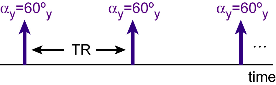
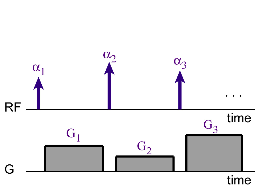
B-1a) Again assume T1=600 ms, T2=100 ms, but we'll assume that there is no off-resonance. Let the sequence repetition time be TR=500 ms. (This should be enough that transverse magnetization dies out before the next excitation.) Begin with TE=1 ms and a flip angle of pi/3, or 60 degrees, about y. Starting with equilibrium, what is the magnetization 1 ms after the first excitation?
Answer: M=[0.8574, 0, 0.5008]'. Matlab Code
B-1b) Make sure you understand the answer to B-1a....!
Now what is the magnetization at time TE after the second
excitation?
Answer: M=[0.6740, 0, 0.3873]'. Matlab Code
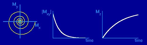
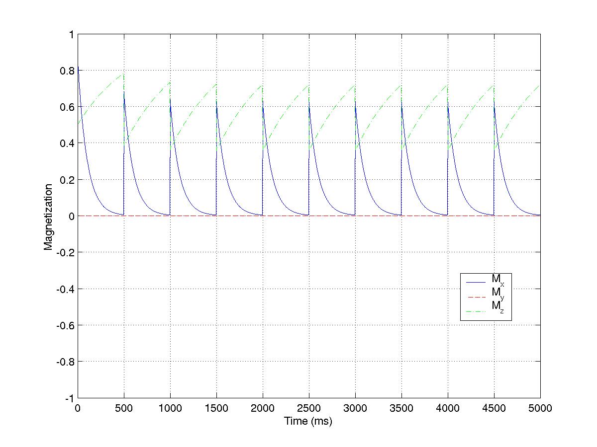
B-1c) Normally we would only be interested in the magnetization
at the echo times (TE). However, for some intuition, let's
look at how the magnetization varies over the first 10 excitations.
Starting at equilibrium magnetization, plot Mx vs time, My vs time
and Mz vs time every 1 ms for 5 s.
Answer: matlab code | view plot
B-1d) After about 2 seconds or 4 excitations, the magnetization
is periodic. We call this a steady state. Sometimes the
magnetization takes much more than 4 excitations to reach a
steady state. Rather than simulating the whole approach to the
steady state, we can explicitly calculate the steady state
magnetization. From the solution to B-1b, we can see that after
exactly one repetition, the magnetization is M1 = Atr*Rflip*M+Btr.
This propagation of magnetization is the same for any repetition,
and in the steady state, M1=M. When M1=M, we can solve the
above matrix equation for M.
What is the steady state magnetization at
the point just prior to the excitation?
Answer: Mss=[0.0042, 0, 0.7203]'. Matlab Code
B-1e) We can calculate the steady-state magnetization at the
echo time (TE) just by multiplying Mss by Rflip, then by Ate and
adding Bte (from B-1a).
However, we can also calculate the steady state at
TE directly by reformulating the "propagation equation,"
(the M1=A*M+B form). Write a
function with the following syntax:
function Mss=sssignal(flip,T1,T2,TE,TR,dfreq). The function
should calculate the steady state magnetization for the given
parameters. Check that sssignal(pi/3,600,100,500,500,0) is the
same as in B-1d). What is the steady state magnetization at
TE=1 ms?
Answer: Mss=[0.6197, 0, 0.3576]' (either way!). | sssignal.m | Matlab Code
B-1f) You could calculate the result of B-1d on paper symbolically
just by neglecting the transverse magnetization prior to the excitation.
This is worth doing... what is the answer?!
Answer: Mss=[0, 0, 0.7224]' Details
B-1g) You could have kept the transverse term in B-1f without that
much more work and got the same answer as B-1d. Alternatively, in
B-1d, multiply the matrix Atr by [0,0,0; 0,0,0; 0,0,1] and you will
get the same answer as B-1f. Try both of these. For the latter
part, just modify sssignal.m, and call the new function srsignal.m.
Answer: srsignal.m
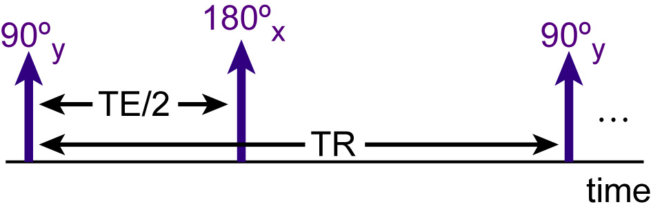
The basic spin-echo sequence consists of a 90-degree excitation about y,
and a 180-degree refocusing pulse about x that is TE/2 after the 90.
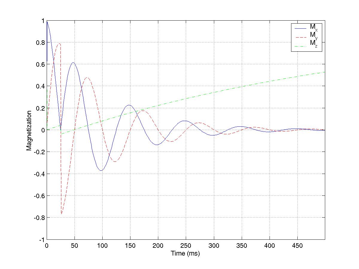
B-2a) Assume T1=600 ms, T2=100 ms, and 10 Hz off-resonance. Plot the magnetization components as a function of time (sampled each 1 ms for TR=500 ms and TE = 50 ms.
Answer: matlab code | view plot Note that the magnetization has a spin-echo at 50 ms -- it points along x at this point.
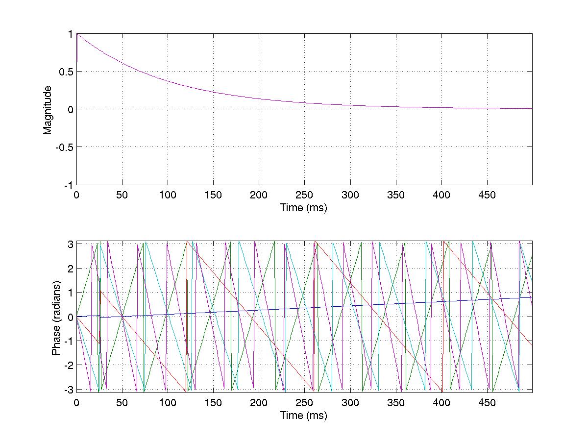
B-2b) To be sure we have a spin echo, take the solution script from
B-2a and plot the magnitude and phase as functions of time. Repeat
this for 10 "spins" with resonant frequencies randomly distributed
between -50 Hz and 50 Hz.
(You can just choose the frequencies randomly, or use the
Matlab function rand.) Plot the magnitude and phase of all of these
spins on one axis. You should see the echo that forms at 50 ms.
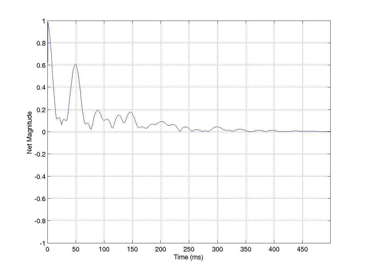
Now plot the magnitude of the complex mean of all of these
signals as a function of time. The meaning of a spin-echo should be
clear!
Answer: matlab code | mag/phase plot | net signal This is a nice simulation of what happens when you have a signal that is the sum of many spins, which is what you actually have. The power of Bloch simulations should be starting to show...
B-2c) The spin-echo sequence also has a steady-state magnetization.
The only difference from B-1 is that you have the extra excitation
refocussing pulse. Write a functon like sssignal.m, but which
includes a 180x pulse at TE/2, and for which the first excitation is
always 90y. You can neglect residual transverse magnetizaton at
the end of the TR -- see B-1f.
Call the funtion sesignal.m. What is Mx for
T1=600 ms, T2=100 ms, TE=50, and TR=1000 ms?
Answer: 0.4822.
| sesignal.m
B-2d) In real life, it is common to use many spin echoes following
one excitation, as 90y - TE/2 - 180x - TE - 180x - TE - 180x - TE - ...
Now modify your function from B-2c to the form:
function M = fsesignal(T1,T2,TE,TR,ETL). ETL is the "echo-train
length" or the total number of spin echoes. The M that this function
returns should be 3xETL (or 1xETL if you are returning the complex
signal like the solution to B-2c), and give the magnetization at each echo.
The sequence is commonly called fast spin-echo (FSE), turbo spin-echo (TSE)
or RARE. What are the signal amplitudes for T1=600 ms, T2=100 ms, TE=50,
TR=1000 ms, and ETL=8?
Answer: [0.3835, 0.2326, 0.1411, 0.0856, 0.0519, 0.0315, 0.0191, 0.0116]
| fsesignal.m
Notice that the amplitude of the first echo is smaller in B-2d than B-2c (why?). If you set ETL to 1, they should be the same.
Spin-echo sequences are commonly used when off-resonance is a
problem. Single-echo sequences can generate good T1-contrast
images. Fast-spin-echo sequences are clinically
the most commonly used method of generating T2-contrast.
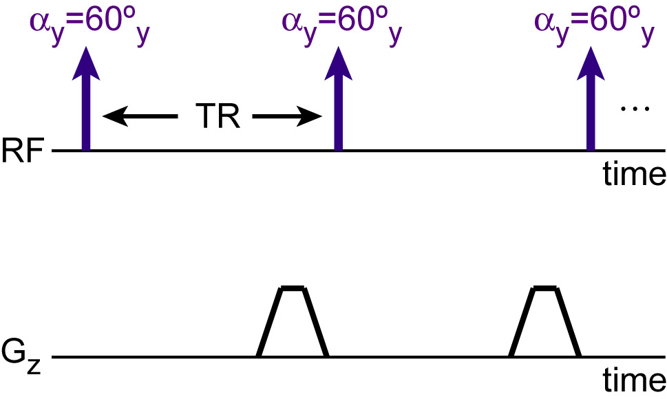
The gradient-spoiled sequence
consists of an excitation and readout as usual. However, at the end of
the sequence is a spoiler-gradient - basically a gradient that tries
to completely dephase the transverse magnetization across a voxel.
Think about what the magnetization does in steady state.
It seems intuitive that we can just neglect the transverse
magnetization at the end of TR, right? Well let's do a more accurate
simulation and see.
B-3a) First, we will want to simulate many magnetizations in
each voxel, separately. We want a function of the form:
function Mss=gssignal(flip,T1,T2,TE,TR,dfreq,phi) where phi is the
angle by which the magnetization is dephased at the end of the TR.
Look at sssignal.m from exercise B-1e. You should be able to modify
it easily to write gssignal.m. After you write this function, find
M=gssignal(pi/3,600,100,2,10,0,pi/2)?
Answer: Mss=[0.1248, 0.1129, 0.1965]'. gssignal.m
B-3b) Okay, now if we were to put a gradient on at the end of TR,
then the angle that magnetization is dephased varies with position
over the voxel. Let's assume that we choose our gradient spoiler so
that there is exactly 4*pi of twist across the voxel. Write a function
of the form function Mss=gresignal(flip,T1,T2,TE,TR,dfreq) that
calculates the average magnetization over, say, 100 points
with the phase varying uniformly from -2*pi to 2*pi. This function should use
gssignal.m from B-3a. What is gresignal(pi/3,600,100,2,10,0)?
Answer: Mss=[0.1157, 0.0000, 0.1801]'. gresignal.m
B-3c) Now for the punch line.
From B-1f, what is srsignal(pi/3,600,100,2,10,0)?
Answer: Mss=[0.0276, 0, 0.0195]'. srsignal.m
The signal (transverse component) is about 4 times higher than the approximation that neglects the transverse decay. You'd also find that it is much higher than the result with sssignal.m, but we'll explore that more in B-4. You could calculate the gradient-spoiled signal symbolically, but it's probably too much fun for one day! (actually it's a lot of work). So what we have seen, again, is that we can run our Bloch simulations to simulate the effect of many spins in a single voxel.
The balanced SSFP sequence simply consists of alpha excitation pulses
spaced TR apart. TR is usually very short, on the order of several
milliseconds.
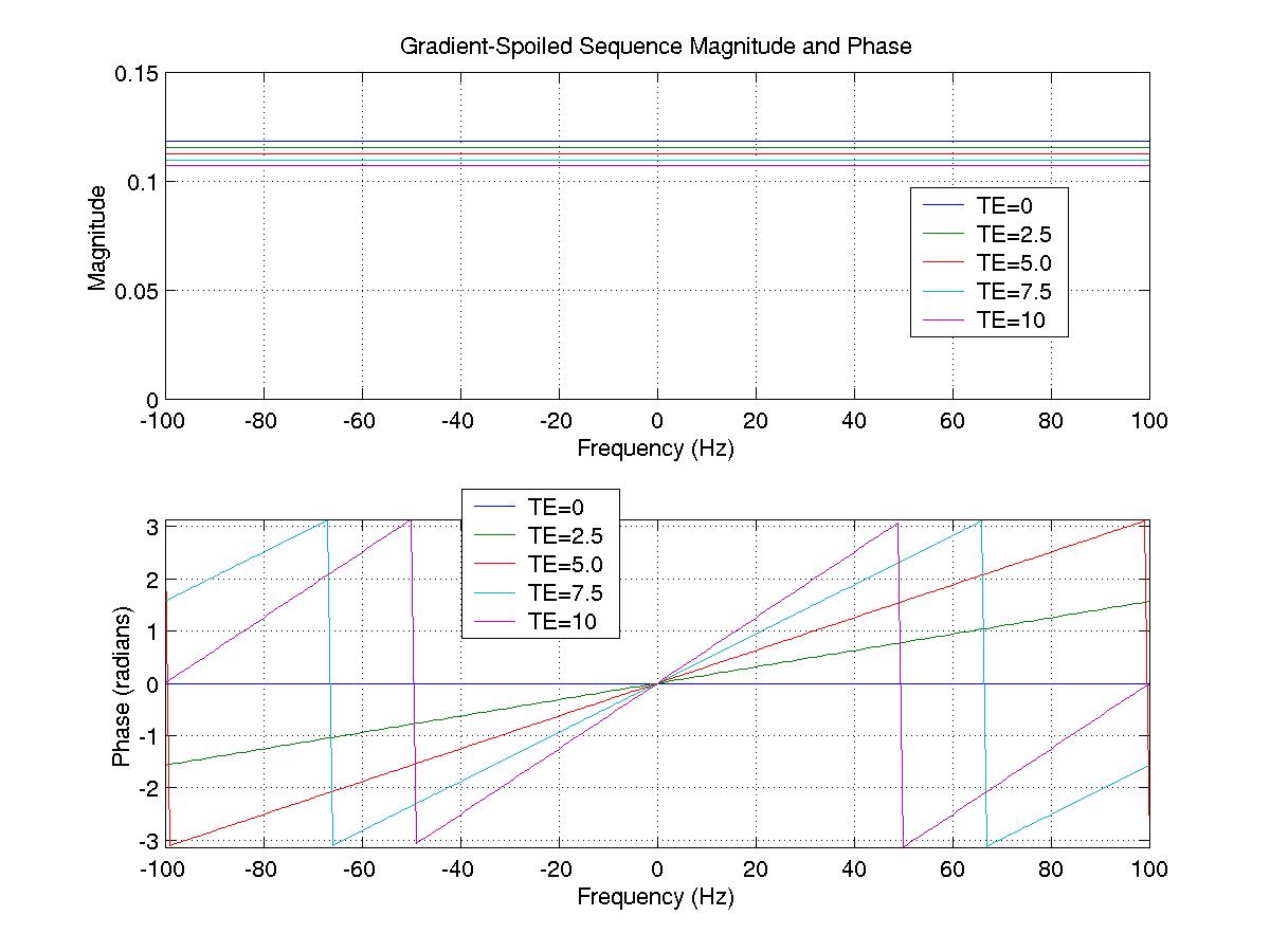
B-4a) Refocussed-SSFP means that the imaging gradients are fully
refocussed. But we haven't put in any imaging gradients yet, so
this is true! The function sssignal.m does, in fact, calculate the
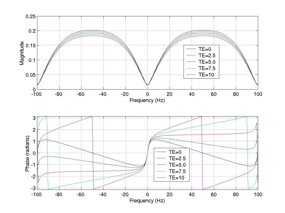
refocussed-SSFP signal. For your first exercise, plot the signal
magnitude and phase for refocussed-SSFP as a function of resonant
frequency. Use T1=600 ms, T2=100 ms, TR=10 ms, and TE=0 ms. Use
a frequency range of -100 to 100 Hz. Then repeat this for
TE=[2.5,5,7.5,10] ms. Note that the TE is really the observation
time. The magnetization dynamics are not affected by the
choice of TE for this sequence.
Answer: Matlab Code | plots
Notice that the magnitude is very sensitive to resonant frequency, and drops slowly over TR due to T2-relaxation. The phase variation consists of regions of linear-phase, with discontinuities of 180 degrees around the magnitude nulls. More importantly, look at the phase at the point TE=TR/2. It is flat from one magnitude null to the next. This means we essentially have a spin-echo, as long as the frequency variation is small.
B-4b) What are the magnitude and phase of the complex-average signal at TE=0?
Compare this with gresignal(pi/3,500,100,10,0,0). Now repeat B-4a, but
plot the gradient-spoiled signal instead of the refocussed-SSFP signal.
ie use gresignal.m instead of sssignal.m
Answer: The mean signal is 0.1176, with a phase of 0. Matlab Code | plots Notice that the signal level of gradient echo (GRE) signal is exactly the same as the mean refocussed-SSFP signal. That makes sense, because the GRE signal was just the average over many spins that had different amounts of phase twist.
Also notice that the GRE signal "dephases" as TE gets bigger. However, the refocussed-SSFP signal actually has a flat phase at TE=5 ms, at least for resonant frequencies between 0 and 100 Hz. The sequences have very different characteristics, and it quickly gets more complex!
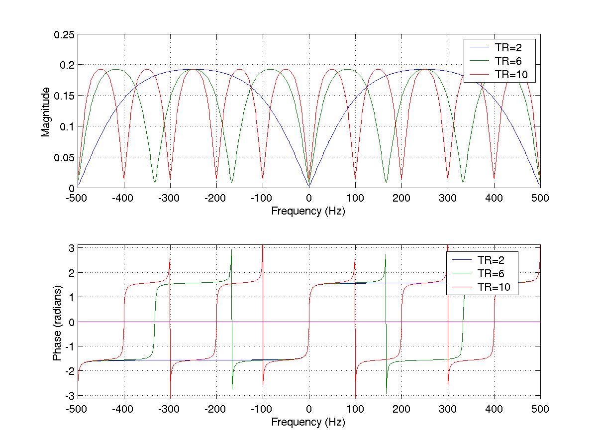
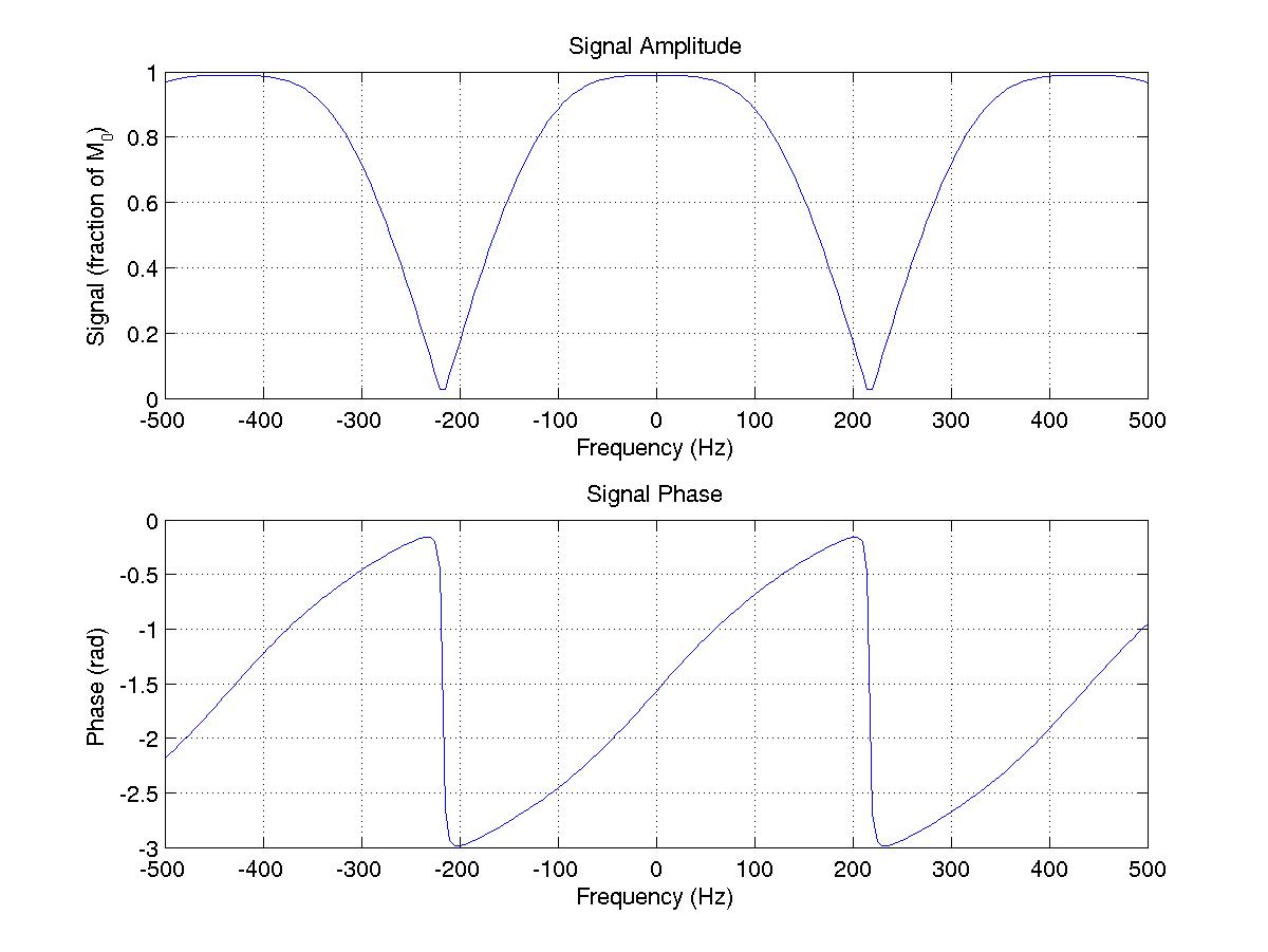
B-4c) Now go back to B-4a again. Plot the magnitude and phase for
TE=TR/2, over the same frequency range. This time vary TR (and TE),
instead of just TE. Do the plots for TR=[2,4,6,8,10], over a frequency
range of -500 to 500 Hz.
Answer: Matlab Code | plots Notice that the signals are periodic. The magnitude nulls are always spaced 1/TR Hz apart. In actual implementations of SSFP, the TR is usually kept less than 5 ms. This means we can tolerate frequency variations of up to about +/-50 Hz without losing too much signal.
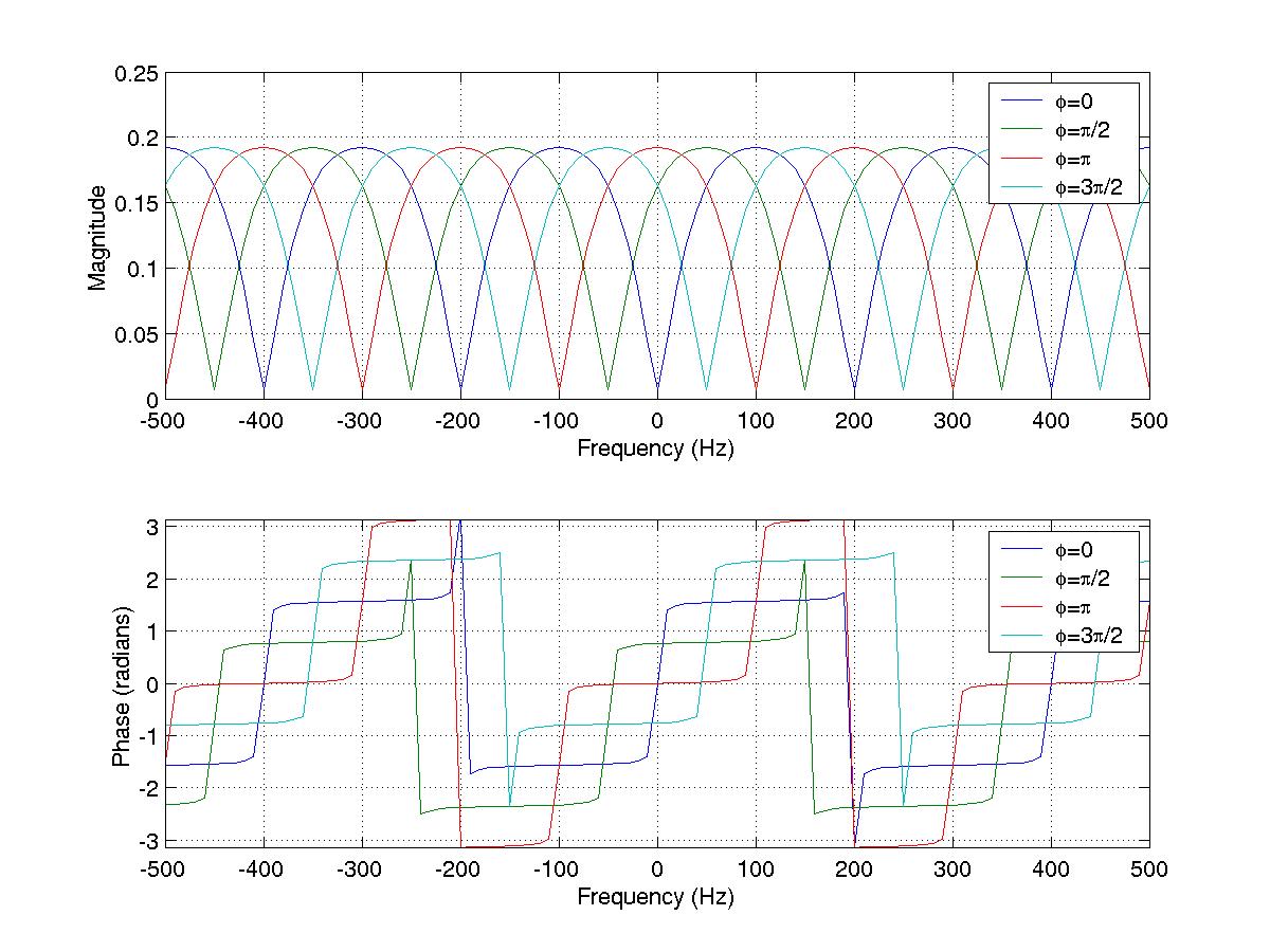
B-4d) The magnitude nulls always occur at 0 Hz. That's not very
desirable, since we ideally have all our magnetization "on-resonance."
We can shift the nulls by using a phase increment on the RF
pulse. This is equivalent to applying a constant rotation of all
magnetization at the end of TR. In fact, just copy gssignal.m to
ssfp.m, because that's what we need! Now plot the signal magnitude and
phase for the same paraemeters as B-4a, but with TR=5 ms, TE=2.5 ms,
and plot for phi = 0, pi/2, pi and 1.5*pi.
Answer: Matlab Code | plots When we apply an increment to the RF phase, we equivalently horizontally shift the refocussed-SSFP frequency response. This can be pretty useful. In "standard" implementations, the RF phase is increased by pi radians on each excitation, so the signal for 0 Hz is not zero. The phase shifts vertically too, but that's not all that important, as we can always multiply the signal by a constant phase.
There's a lot more that we could look at with SSFP. Compared with FSE or GRE, the signal is pretty complicated. We'll leave that until a future section though!
An RF-spoiled sequence includes gradient spoiling, but in addition, the phase of the excitation pulse changes on each excitation:
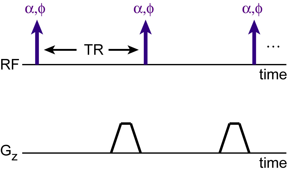
The RF-spoiled sequence is similar to the gradient-spoiled
sequence use alpha to indicate the flip angle, and phi to
represent the phase of the excitation.
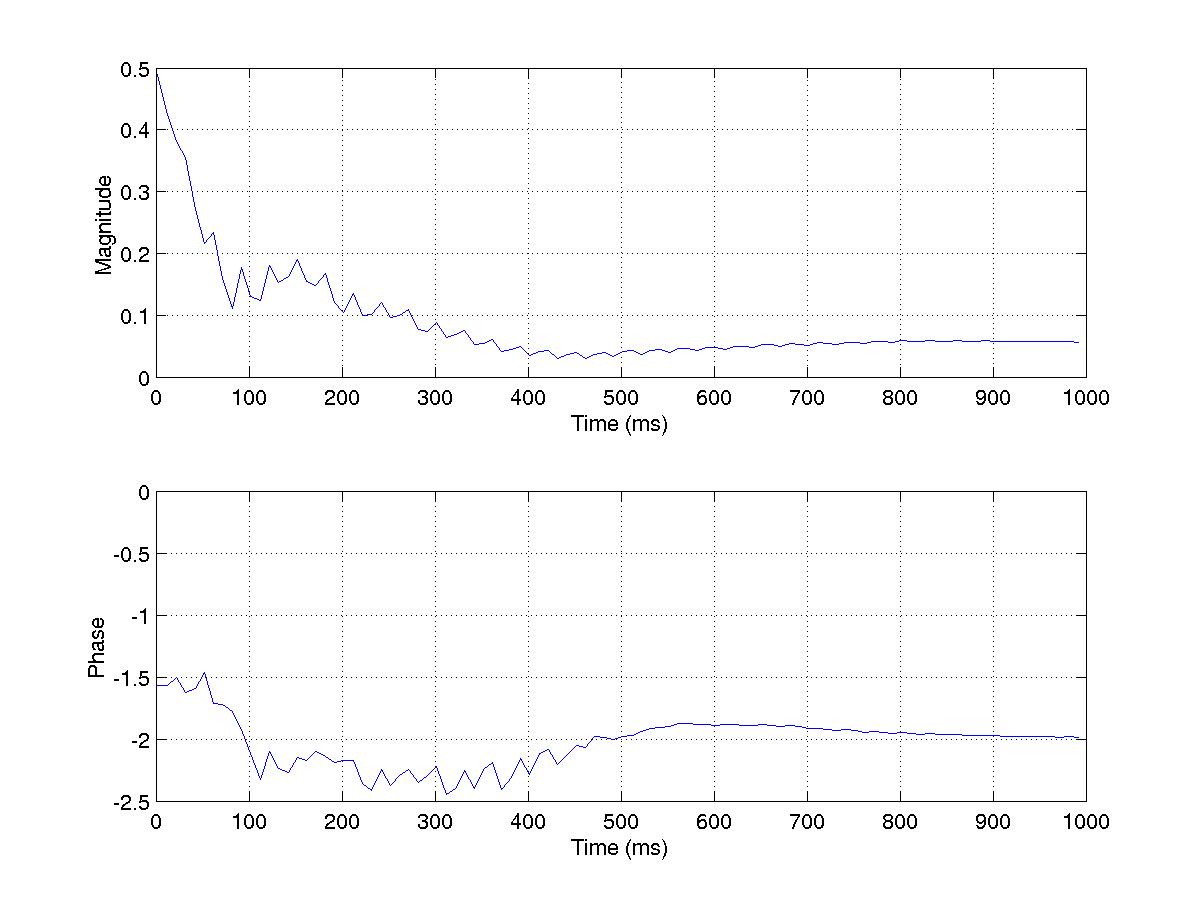
B-5a)
The common way to vary the phase is to increment the
excitation phase (phi) by I on each excitation.
The increment, I, is
increased by 117 degrees on each excitation as well, so the RF phases
for the first 5 excitations are 0, 117, 351, 702, 1170 degrees.
(The phase of the last RF pulse is subtracted from the signal phase
on each excitation as well.)
Simulate the signal magnitude and phase as a function of excitation number, starting at 0. Again, use T1=600 ms, T2=100 ms, TR=10 ms, TE=2 ms and a 30-degree flip angle. Do the simulation for 0 Hz off-resonance. Plot the magnitude and phase at TE for the first 100 excitations.
Answer: Matlab Code | plots Notice that after many excitations, the magnetization has reached a pseudo-steady-state. We will look at this more.
B-5b) Take the code from the last exercise and convert it to a
function of the form:
function Msig=spgrsignal(flip,T1,T2,TE,TR,dfreq,Nex,inc) where
Nex is the number of excitations, and inc is the RF phase increment.
(Use pi*117/180 for inc for now).
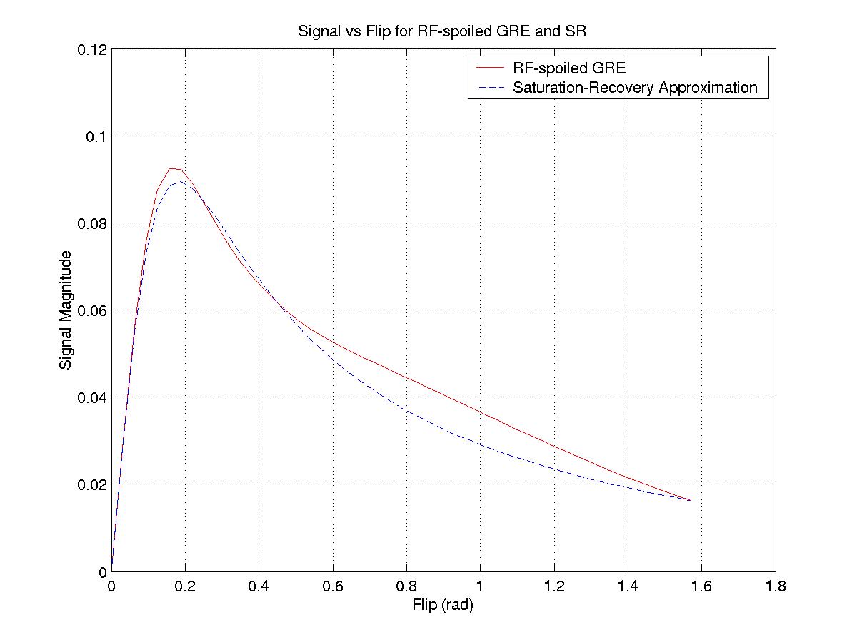
Using your function, plot the signal magnitude vs flip angle for
T1=600 ms, T2=100 ms, TR=10 ms, TE=2 ms, dfreq=0 Hz and Nex=100.
On the same plot, plot the signal magnitude using srsignal.m.
Answer: spgrsignal.m | Matlab Code | plots The plots agree quite well. RF spoiling is commonly used in sequences where T1-contrast is desired.
Hint! -- For this section, you will be using the .m functions that you wrote in the previous section. It would be worth modifying them to return the complex signal - ie Mx+i*My as well as the magnetization vector. Then for this section you can just use the Matlab function fplot for most of the exercises!
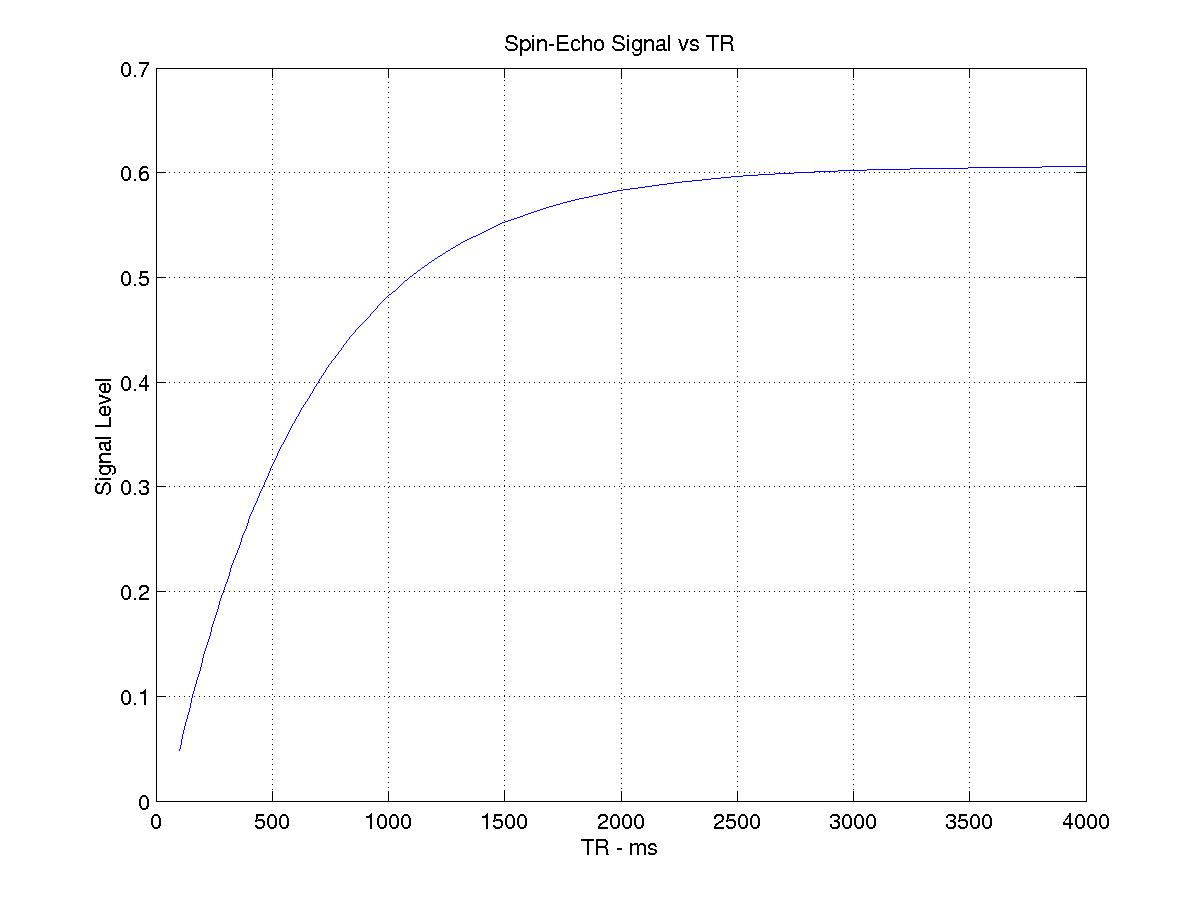
C-1a) Using sesignal.m, plot the spin-echo signal level with TE=50 ms, as
a function of TR, with TR varying from 100 ms to 4000 ms.
Answer: Matlab line: fplot('abs(sesignal(600,100,50,x,0))',[100,4000]); plot
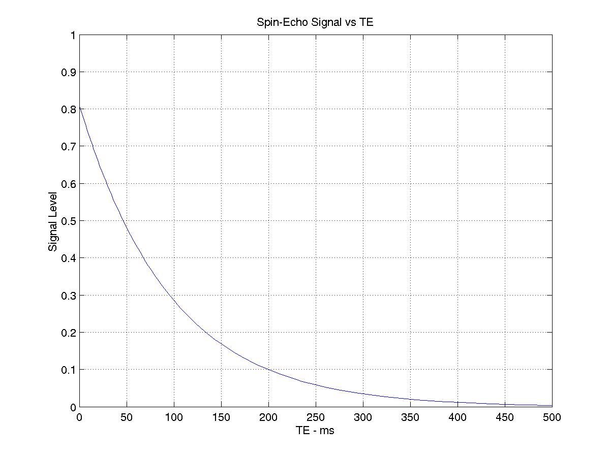
C-1b) Plot the spin-echo signal level as a function of echo time for
TR=1000 ms.
Answer: Matlab line: fplot('abs(sesignal(600,100,x,1000,0))',[0,500]); plot
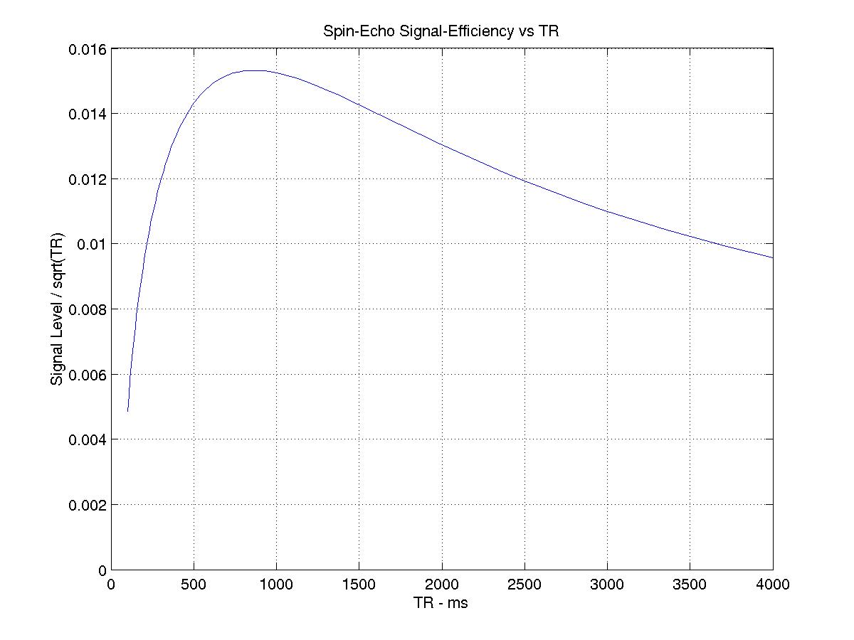
C-1c) In C-1a and C-1b, you notice that the highest signal
is when TR is infinite, and when TE is zero. So what are the
design choices? The first is signal-efficiency, or SNR-efficiency.
Remember that in imaging, your SNR is proportional to the square-root
of total readout time. Let's assume that our readout time per TR is
constant. Repeat C-1a, but instead of just plotting signal level,
plot the ratio of signal level to square-root of TR.
Answer: Matlab line: fplot('abs(sesignal(600,100,50,x,0))/sqrt(x)',[100,4000]); plot
You now have an optimal TR on the plot. Given a finite amount of time, and the other parameters, choosing TR=860 ms gives you the best SNR efficiency.
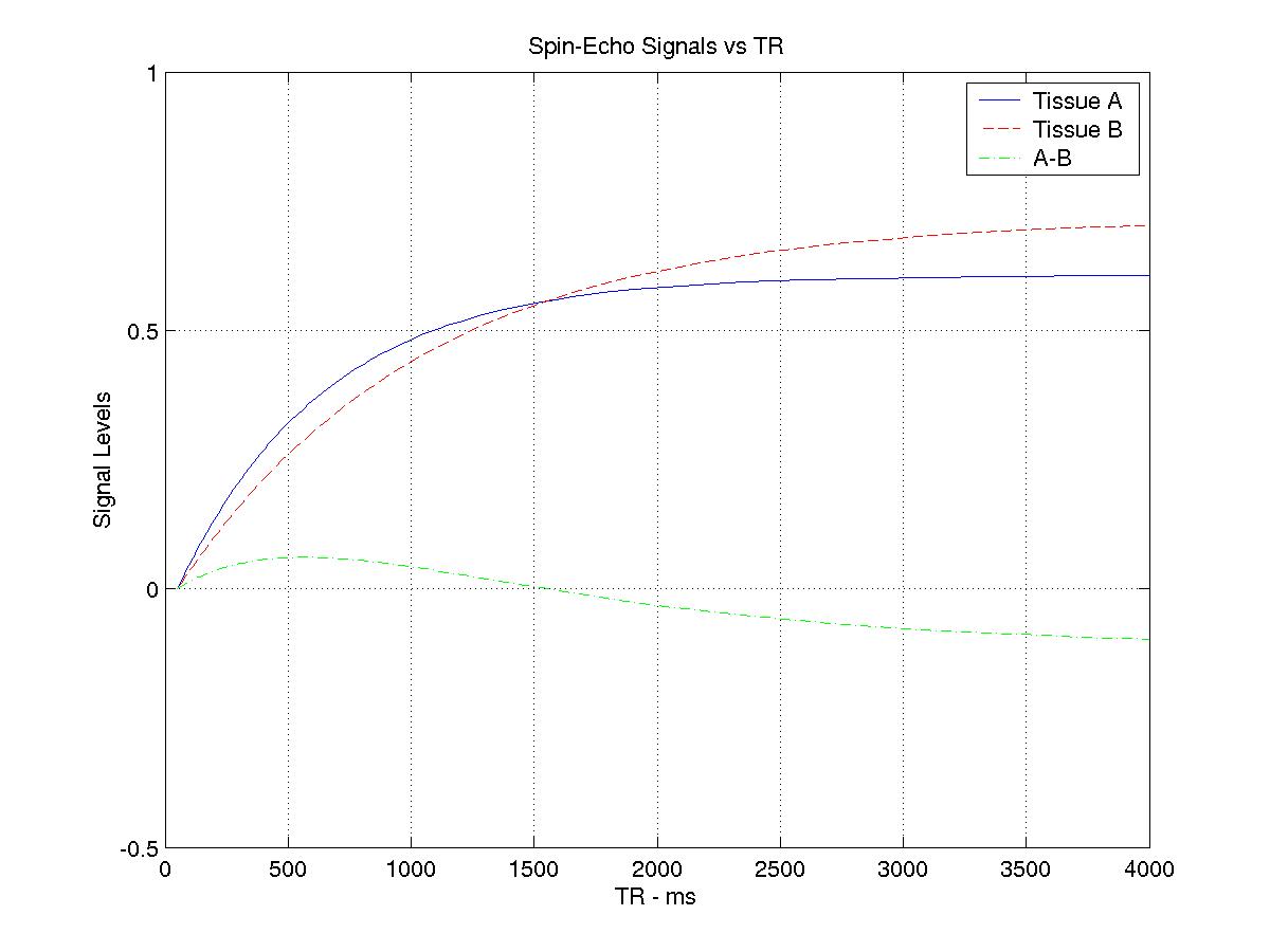
C-2a) So far, our "tissue" has been characterized by T1=600 ms and T2=100 ms. Let's call this tissue A. Now we'll also introduce tissue B that has T1=1000 ms and T2=150 ms. Again we will use a simple spin-echo sequence, ie sesignal.m. Repeat C-1a, but plot the signal for both tissues. Also plot the difference between signals as a function of TR, on the same plot.
Answer: Matlab Code | plot Notice that Tissue A is favoured at shorter TR values, because it has the shorter T1.
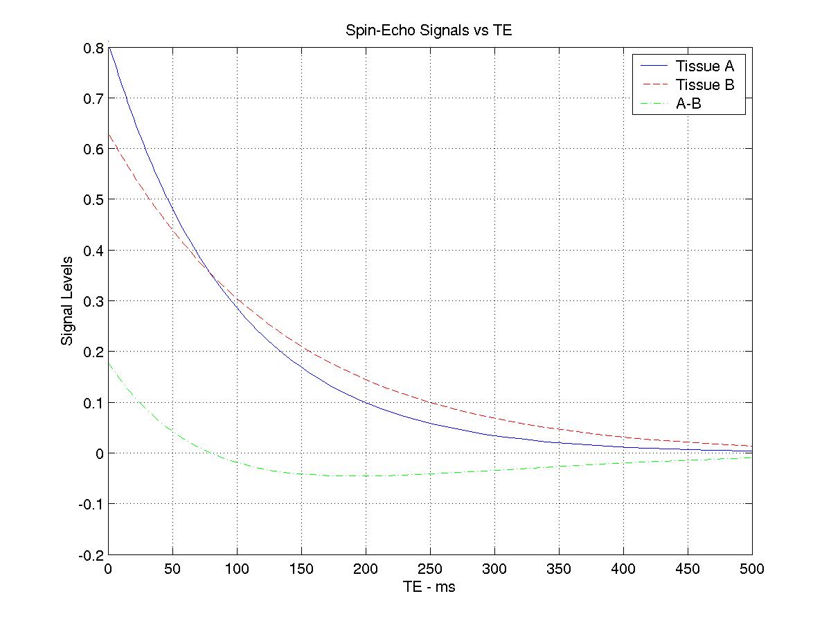
C-2b) Now repeat C-1b, but again plotting both tissues and the
signal difference.
Answer: Matlab Code | plot Tissue B is favoured at longer TE values because it has a longer T2.
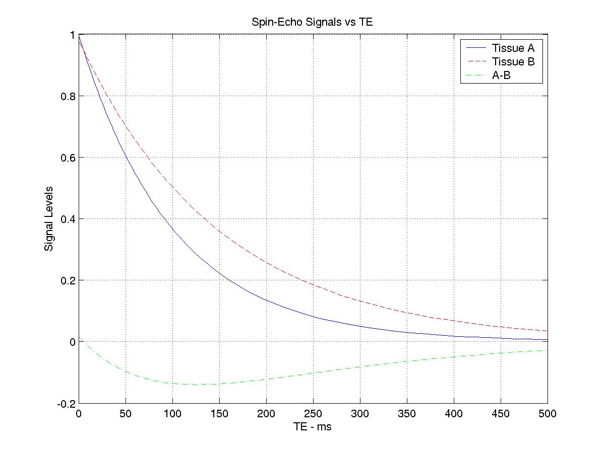
C-2c) Why does the contrast curve cross in C-2b? At low TE values,
we get T1-contrast. To avoid this, and get pure T2-contrast, we
really should increase the TR. Repeat C-2b for TR=4000 ms.
Answer: Matlab Code | plot We could have said this in C-2a as well... in order to get pure T1-contrast, we should minimize TE. We'll leave that for now though, but if you like, try C-1a with TE=10 ms to see the difference.
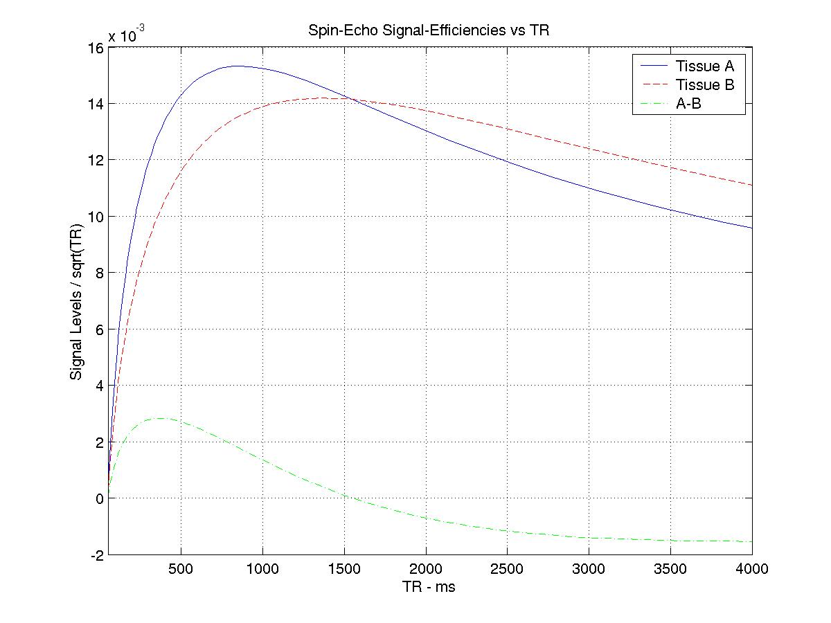
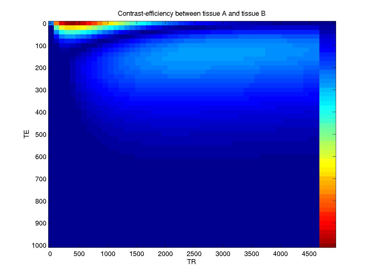
C-2d) There is also a quantity called contrast-efficiency. That's
just the difference in signal-efficiency of two tissues. Repeat
C-2a, but normalize all three quantities on the plot by the square
root of TR.
Answer: Matlab Code | plot Interesting, now there are three different TR values, each optimal in a different sense. The contrast peak is where there is the most T1-contrast (Tissue A is higher). We could have used a different TE and done this same test -- notice that the T2-contrast efficieny is still increasing at TR=4000, and we didn't even use the best TE for that. Also, if we did optimize T2-contrast efficiency, we are not close to the signal-efficiency maximums. This is the reason for multi-echo sequences like FSE. We'll explore FSE a bit later.
Things are getting complicated, just because we added a second tissue. In real life we often have to generate contrast between two or three different tissue types. Magnetization-preparation can be useful for this -- we'll look at that later.
C-3a) In C-2a, we saw that a simple spin echo sequence can
provide T1 contrast. Here we use the same two tissues,
tissue A with T1=600 ms and T2=100 ms, and tissue B with
T1=1000 ms and T2=150 ms. Using sesignal.m, what TE and TR give
you the maximum contrast-to-noise efficiency? What type of
contrast is this sequence producing? Assume for now
that your RF pulses and readout can have zero-duration(!)
To be sure, write a function that plots CNR-efficiency as
a function of both TR and TE. (You can use image(x,y,C) in
Matlab...)
Answer: You should find that TE=0 ms, and TR=375 ms. This is a T1-contrast sequence. Matlab Code | plot. Try changing the range of TE and TR in the Matlab code to be sure.
C-3b) If you insisted on T2-contrast, what TR and TE give you the
maximum CNR efficiency?
Answer: From the plot in C-3a, TR is about 3000 ms, TE is about 130 ms.
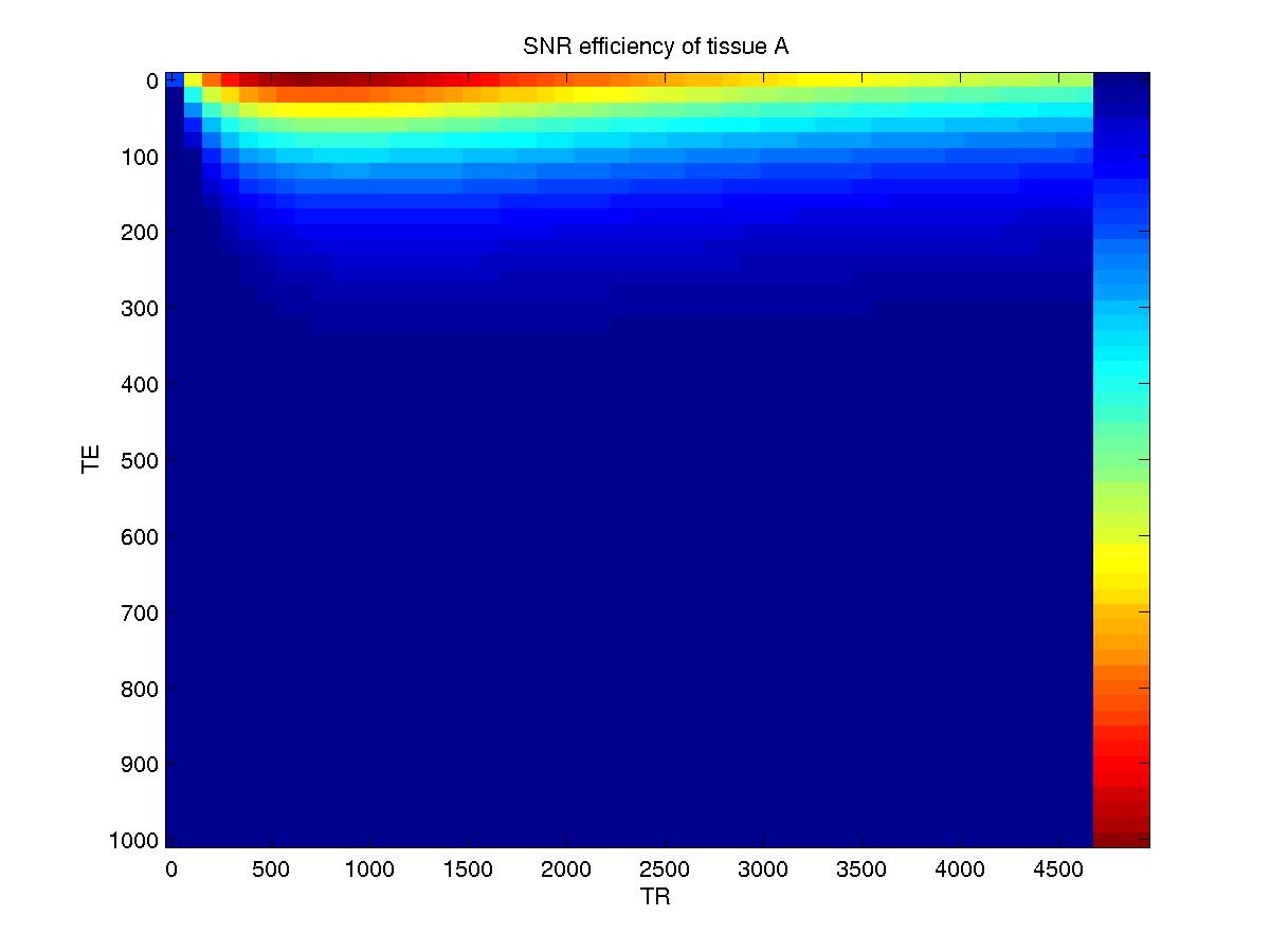
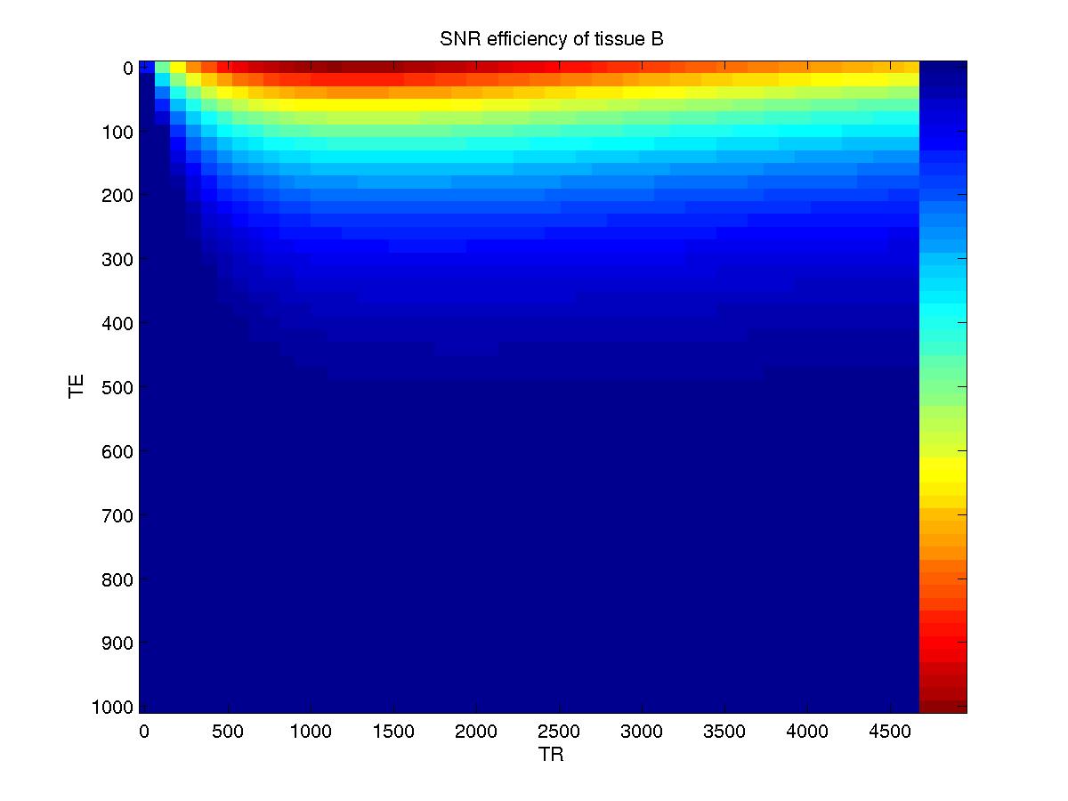
C-3c) Modify the code in C-3a to plot the SNR efficiency for tissue A.
Then repeat this for tissue B. What can you say about the SNR efficiency
at the points of optimal T1 and T2 contrast-efficiency.
Answer: plot A | plot B | Matlab Code As in C-2, we see that the SNR efficiency is not very high when we have the best T2 contrast-efficiency. Multi-echo sequences can help to address this problem.
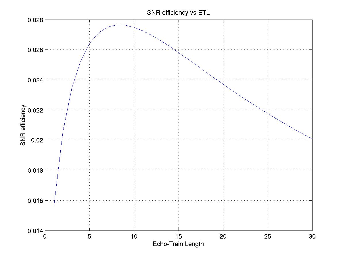
C-3d) Consider a spin-echo sequence with N echoes. Now we take the
signal as the sum over the N echoes. First, if the signal amplitude
were the same on all echoes, how would you expect the SNR to vary with
N? Now, for tissue A, and an inter-echo spacing of TE=15 ms, and TR=3000 ms,
plot the SNR efficiency as a function of echo-train length (ETL), for
ETL=[1:30].
Use fsesignal.m that you wrote in B-2d.
Answer: If the signal is constant, SNR goes up as sqrt(ETL) because signal goes up with ETL and noise with sqrt(ETL). plot | Matlab Code
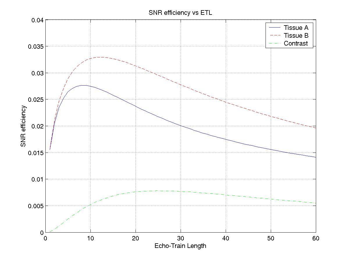
C-3e) Okay. So we should have a peak with an ETL of 7. Now modify the
code from C-3d to plot the SNR efficiency of tissues A and B, and the
CNR efficiency as a function of echo-train length. Use the same TE and
TR as in C-3d, but plot for ETL=[1:60].
Answer: plot | Matlab Code
Notice that the optimal CNR efficiency is when the number of echoes is
24. That means the echo train extends for 360 ms. Not quite the same
as our answer in C-3b, but there is a different effect from averaging.
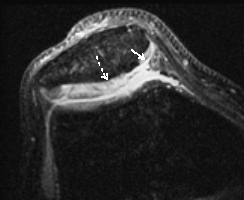
C-3f) There are two ways to use the signal from multiple echoes. One is to acquire a separate image corresponding to each echo. This seems like a nice way to measure T2 across an image (though in practice it isn't the most accurate method). The second, which is FSE, is to acquire different spatial frequencies from different echoes. Although FSE is much faster (how much?) than forming complete images, the fact that different spatial frequencies have different contrast can be a problem.
As an example, look at this
FSE image of knee cartilage
acquired with TR=3200 ms, TE=15 ms and ETL=4 ms.
The cartilage (which has a T2 of 30 ms) is blurred (surface shown by the
dashed arrow), because the low spatial frequencies are acquired on
the earlier echoes. By the third
or fourth echo, the cartilage signal has decayed significantly, so there
is a low-pass filtering effect. There is some synovial fluid in the
image as well (solid arrow), which has a T2 of over 200 ms.
Notice that the synovial fluid is not blurred like the cartilage.
(C-3f was just a reading exercise...!!).
C-3g) Now if we use the multi-echo technique to generate an image for each echo, we could try to fit the decay to determine T2 in each pixel. This is very useful, actually. However, the problem is that there is also some loss from each 180-degree refocussing pulse being imperfect. As an exercise, if we had a T2 of 200 ms, and we model each 180-degree pulse as retaining 95% of the signal, what T2 would you measure by fitting the decay across images? Assume no noise, and an inter-echo spacing of 15 ms.
Answer: -15/ln(0.95*exp(-15/200)) = 119 ms.
A much better (but slower) method is to use a single spin echo for each image and vary the imaging time.
There are many more details to spin-echo and FSE sequences. However, the important things we have shown here are that spin-echo can give us T1-contrast, and FSE is better for T2-contrast as it has high efficiency.
C-4. RF-Spoiled Gradient Echo (SPGR)
SPGR sequences are a popular method of generating
T1-contrast in rapid sequences. Here we explore the
contrast characteristics of SPGR.
C-4a) We will again use tissue A and B from C-3.
Modify the code in C-3a to plot the CNR efficiency
of SPGR as a function of TR and flip angle.
Use TE=5 ms. What TR and flip angle give you the
peak CNR efficiency?
C-4b) Now repeat C-3c for SPGR. That is, plot the
SNR efficiency for tissue A and tissue B on separate
plots as functions of TR and flip angle. Again use
TE=5 ms.
C-4c) Compare the SNR efficiency and CNR efficiency
of SPGR to spin echo. You may need to modify the code
used in C-3 so that the colour scale is the same in the
C-3 and C-4 plots. Which sequence gives you the best
SNR efficiency? CNR efficiency?
C-5. Gradient-Spoiled Gradient Echo (GRE)
GRE techniques are very common. It is useful to compare
their contrast characteristics to the other sequences
here. As with SPGR, we tend to want to keep the TE at
a minimum because of T2* effects.
C-5a) Repeat C-4a, with identical parameters, but for GRE
instead of SPGR.
C-5b) Repeat C-4b, but for GRE.
C-5c) Repeat C-4c comparing GRE to spin echo and SPGR.
C-6. Refocussed Steady State Free Precession (SSFP)
SSFP, as we discovered in B-4, can produce a higher signal
than GRE, but is sensitive to off-resonance.
C-6a) Write a function ssfpavsignal that returns the SSFP signal
for given parameters, but averaged over a uniform distribution
of off-resonance values deltaf that is one of the parameters,
but centered on the frequency that is passed.
Test this function by plotting the
signal as a function of frequency for tissue A with TR=5 ms, TE=2.5 ms,
and deltaf = [10, 20, 50, 100] Hz.
C-6b) For the next three exercises we assume that we have a +/-30 Hz
range of resonant frequencies. First repeat C-4a with ssfpavsignal
plotting CNR efficiency as a function of flip angle and TR, for
TE=TR/2. Use a range of TR values from 2 to 20 ms.
C-6c) Repeat C-4b using ssfpavsignal and the ranges of C-6b.
C-6d) Now compare SNR efficiency and CNR efficiency of SSFP with
the other sequences
Upcoming Exercises (Bug me if you got this far and need more!)
|
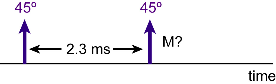
F-1a) First, let our "selective excitation" consist of two
consecutive delta pulses as shown(ie two discrete rotations) that
are spaced 2.3 ms apart. The rotations both have a tip
angle of 45 degrees (pi/4) and a phase of 0. Plot the
transverse magnetization (magnitude and phase)
immediately after the second delta pulse, over the resonant
frequency range [-500 Hz, 500 Hz]. You can assume
T1=600 ms and T1=100ms.
Answer: plot | Matlab Code |
|
|
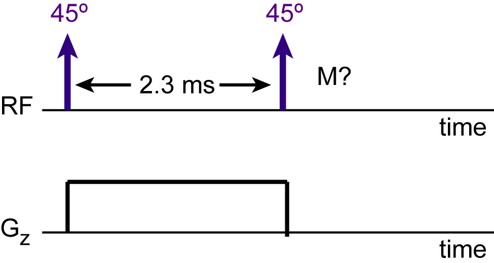
F-1b) You should see that the signal phase is almost linear.
The excitation in F-1a) is selective in resonant frequency.
Now let's assume that there is no variation in resonant frequency.
Instead we turn on a gradient of strength 0.1 G/cm (in the x direction)
for the whole excitation of F-1a.
Given that the gyromagnetic ratio is gamma=4258 Hz/G,
plot the signal amplitude as a function of position, over
a range [-2 cm, 2 cm].
Answer: plot | Matlab Code
|
|
|
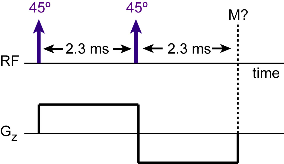
F-1c) Now you see the same pattern, but because we turned on
the gradient, the selection is spatially selective.
It would be nice to get rid of the linear phase across the
slice, though. We can do this by playing half the negative
gradient area after the last RF pulse. Repeat the simulation
of F-1b), but let the gradient be -0.05 G/cm after the last RF
pulse for 2.3 ms, and plot the magnetization as a function
of spatial position 2.3 ms after the last RF pulse:
Answer: plot | Matlab Code |
|
The extra gradient in F-1c was called a refocusing gradient,
because the magnetization is refocused across the spatial
direction. Notice that the magnetization profile is
approximately a cosine, along y.
|
Up until now, all of the RF pulses that we have worked
on are discrete "delta" pulses. In reality, RF pulses
are finite-duration, and limited in amplitude. To exactly
simulate RF pulses with gradients, we need to calculate
the effective B field at any point. However, a simpler
method is the hard pulse approximation, where the
RF and gradients are sampled finely in time. Then the
RF and gradient are applied in the same manner as
in F-1b and c.
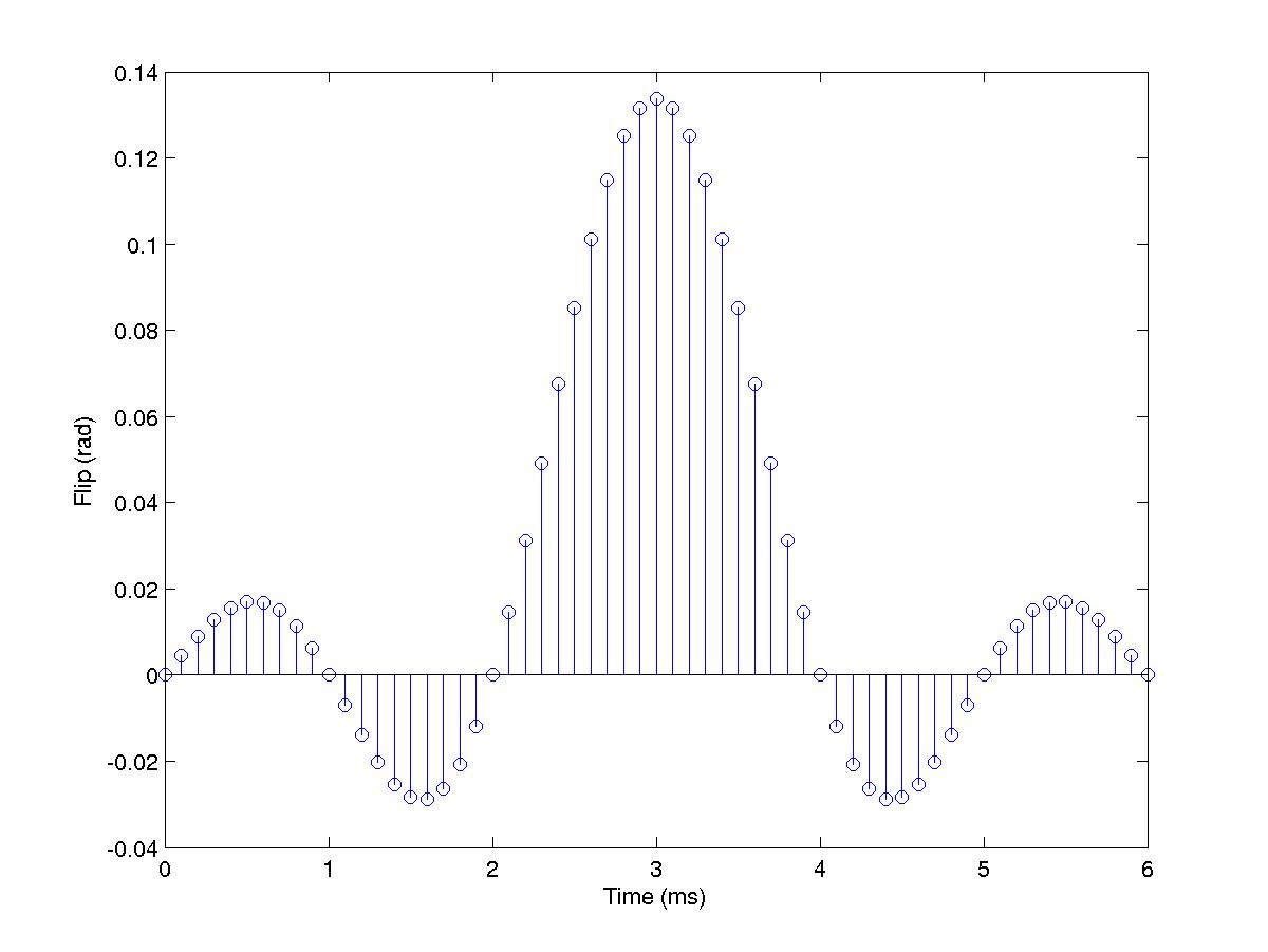
F-2a) Given a B1 field of the form B1(t)=(0.06 G)sinc[(t-3ms)/1ms] for t=[0,6ms], where sinc(x) = sin(pi*x)/pi*x, plot the discrete rotations (as a function of time) if the RF pulse is sampled every 100 us. What is the flip angle for on-resonant magnetization when no gradient is applied? Answer: plot | Matlab Code | The net flip is 82 degrees.
|
Hard pulse approximation. The RF rotations and rotations due to gradients (or precession) are applied sequentially. (Non-zero gradients are not used until F-3.) |
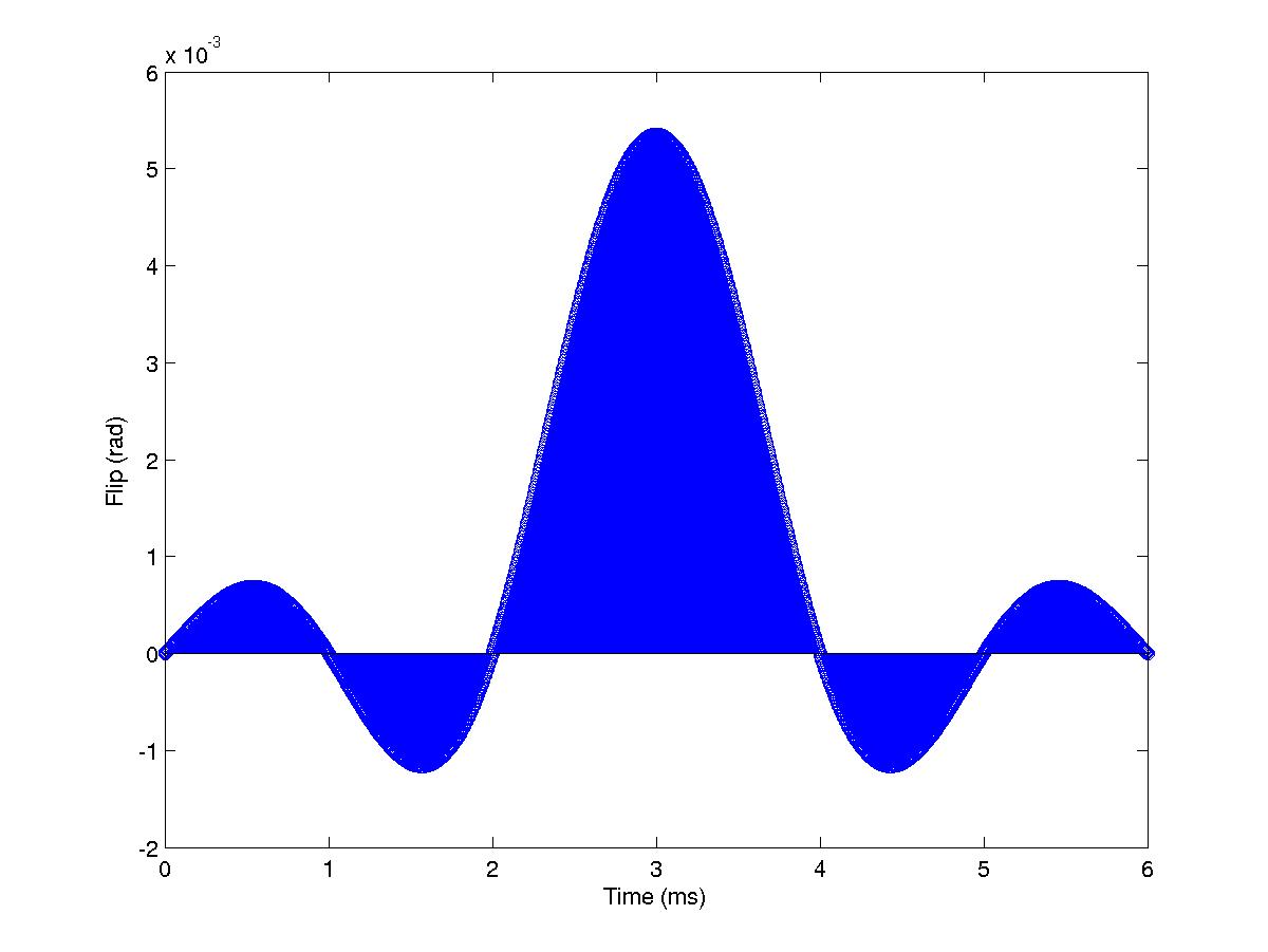
F-2b) Repeat F-2a, but now sample B1 every 4 us (this is typical
on scanners). What happened to the amplitude of the discrete
tips?
Answer: plot | Matlab Code | The net flip is still 82 degrees, but the individual flips are much smaller.
F-2c) Now to the hard pulse approximation. Look back at
F-2a, and simulate the discrete rotations as if they were
deltas (in time). Between the rotations, simulate off-resonance
precession. Repeat the simulation over a range [-1000 Hz, 1000 Hz]
with the RF discretized at 40 us intervals.
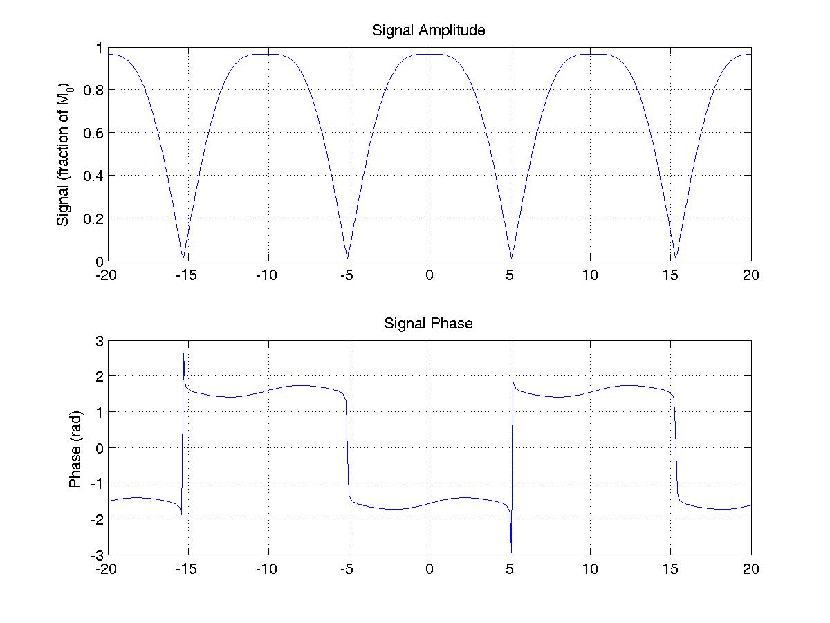
Answer: plot | Matlab Code | We have selectively excited a rect() function profile, the Fourier transform of the sinc(). Note that like F-2a, there is a linear phase across the spectrum.
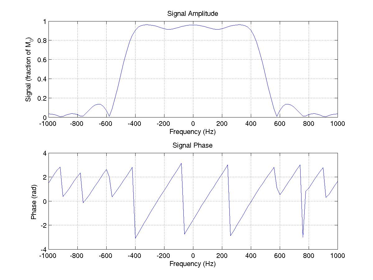
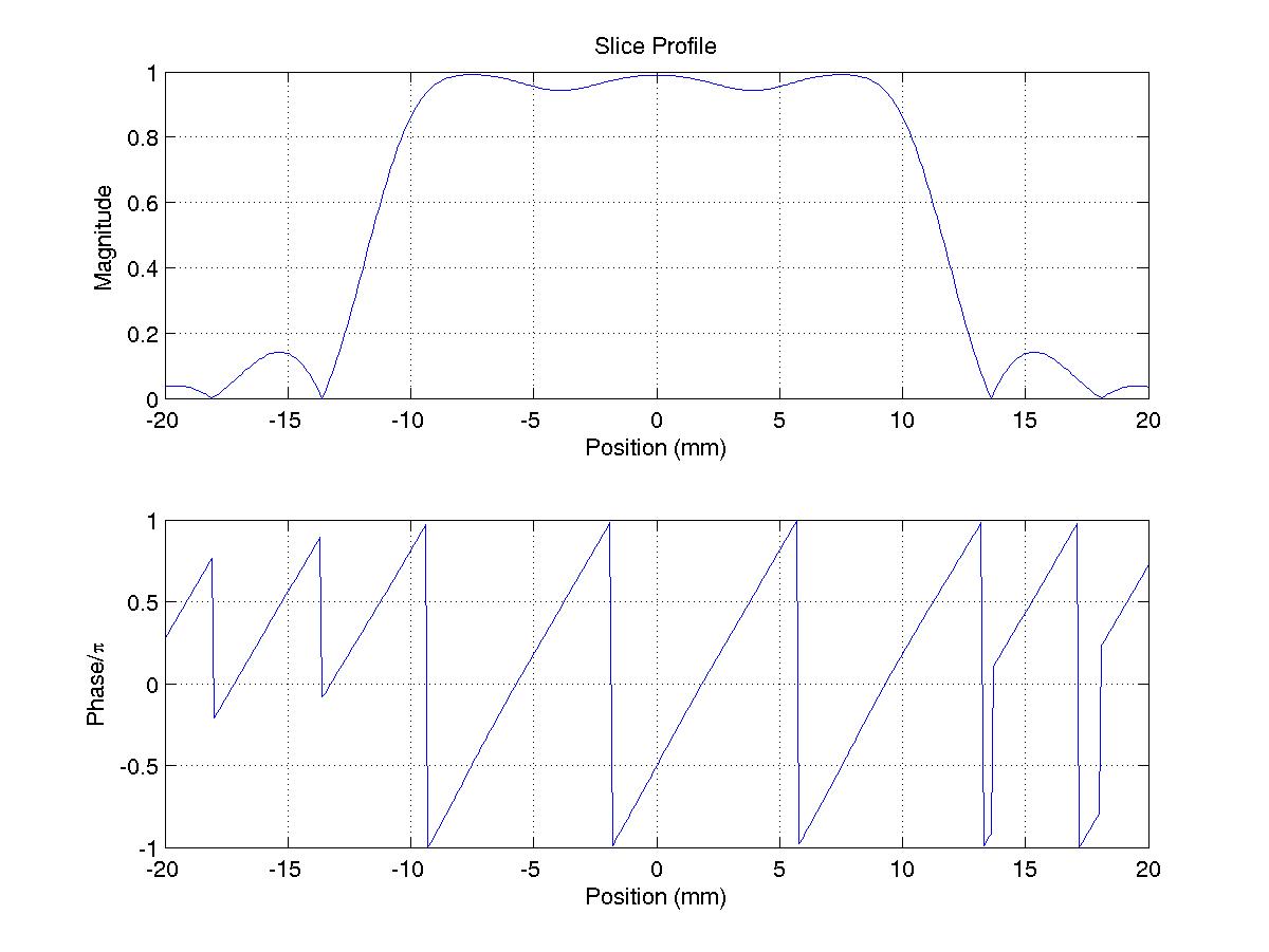
F-3a) For each discrete point, we play gradient-induced precession for half the sample time, then do the RF rotation over the full sample time, then play the gradient for half the sample time. Write a function of the form [m,msig]=sliceprofile(rf,grad,t,T1,T2,pos,df) where rf, grad and t are vectors representing the B1 strength (G), gradient strength (G/cm) and time (s). T1, T2 and df are the relaxation times and offset frequency. pos is a vector of positions (mm) for which to calculate the profile. m and msig are 3xN and 1xN arrays of the magnetization and signal at each point in pos.
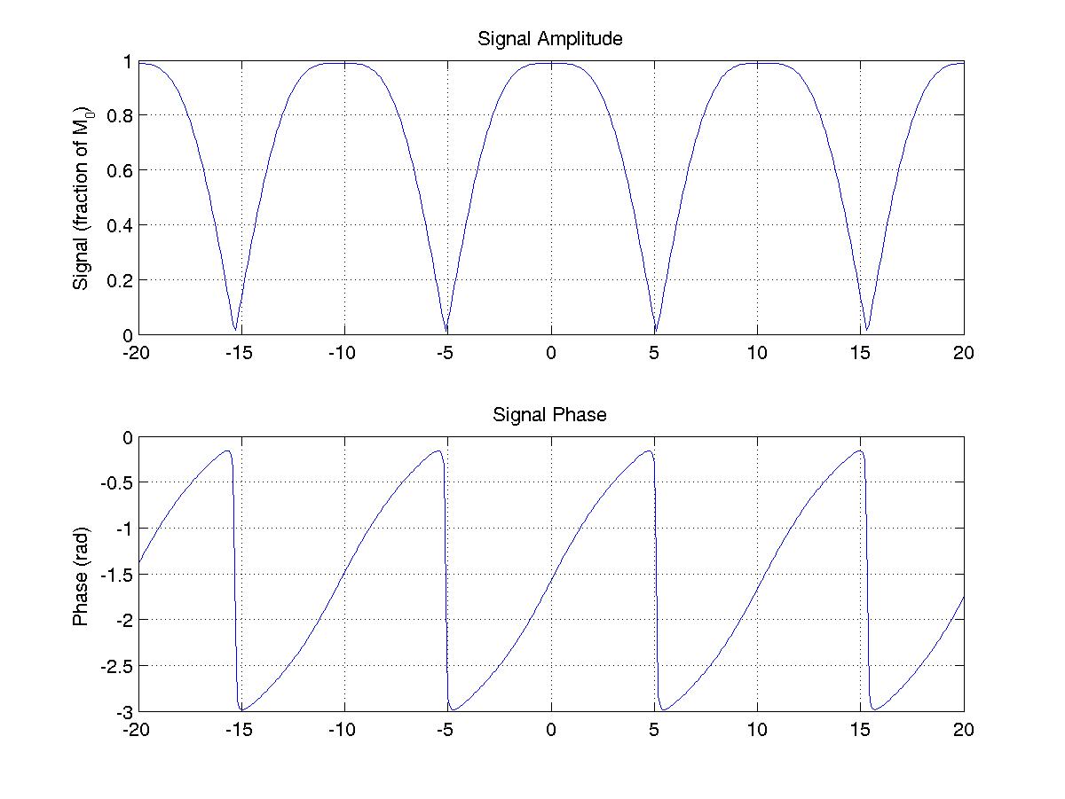
Test this function by running the following commands, then plotting
the magnitude and phase of msig:
t = [0:.0001:.006];
x= [-20:.1:20];
[msig,m]=sliceprofile(.05*sinc(1000*t-3),0.1*ones(size(t)),t,600,100,x,0);
Answer: plot | sliceprofile.m
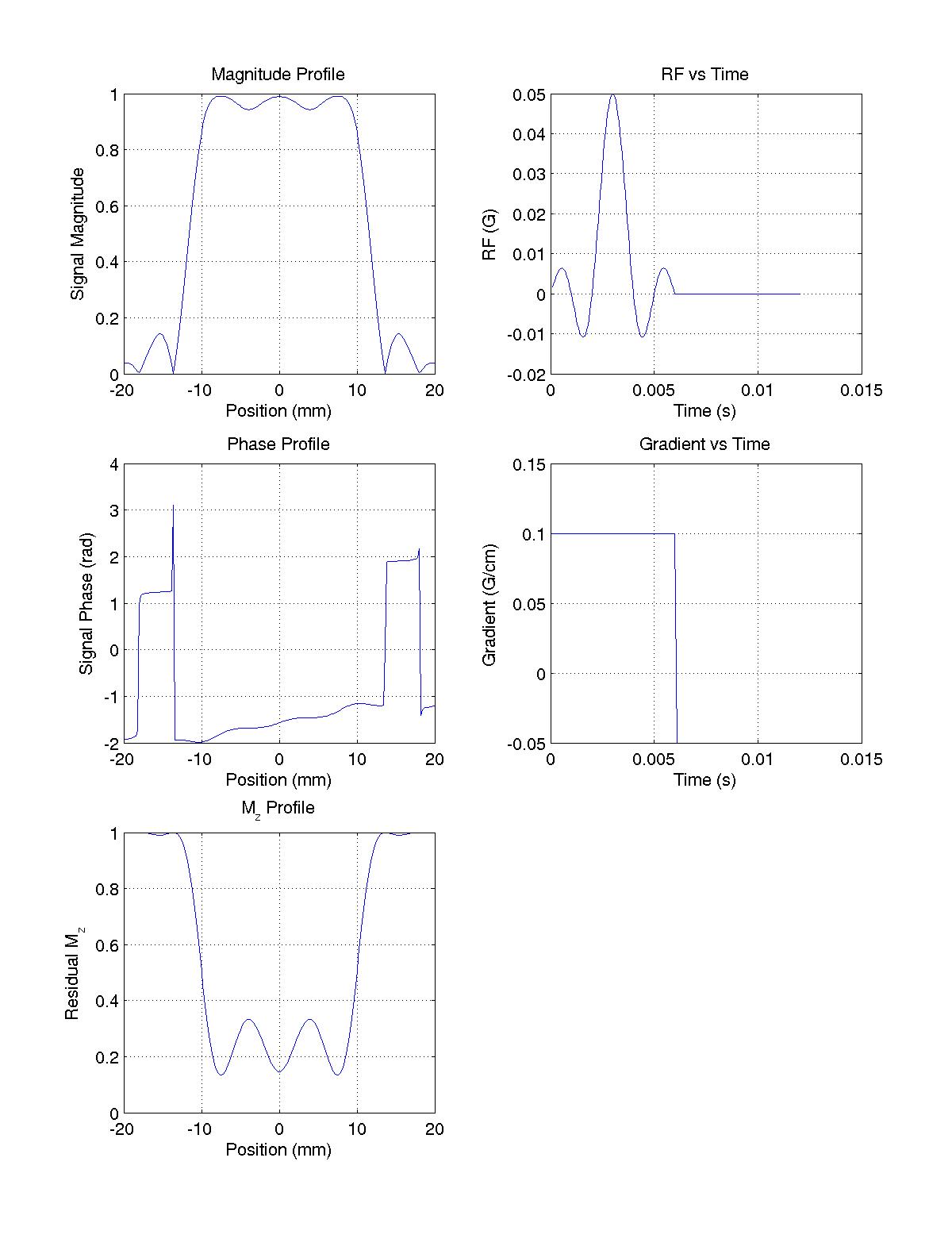
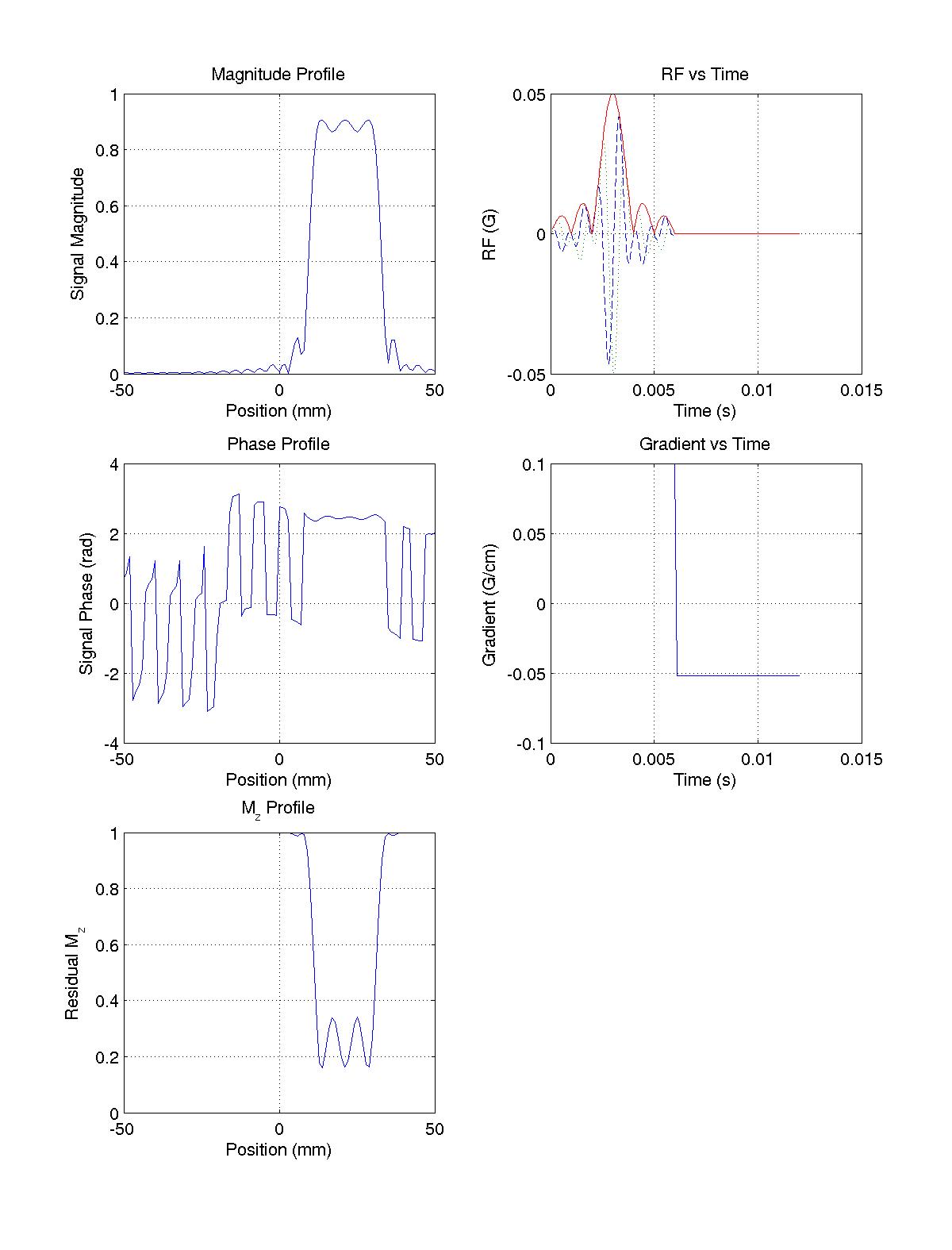
F-3b) Now test the function some more by generating
the RF and gradient waveform used in F-3a. However,
append a "refocusing" gradient to the gradient waveform,
and make the RF zero for this time. Simulate the RF
and gradient over the same x-vector as F-3a. Plot the
magnitude and phase of the signal as a function of
position.
Also plot the z-component of
the magnetization at the end of the sequence.
Finally, plot the RF and gradient waveforms as
functions of time.
Answer: plot | Matlab Code
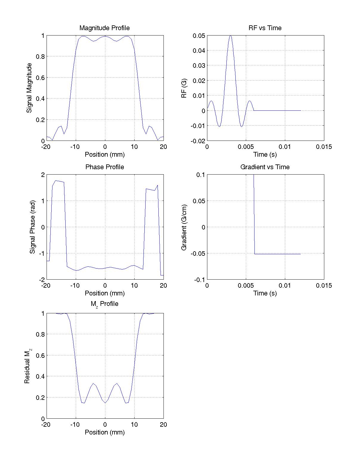
F-3c) Notice that the magnetization is not perfectly refocused.
We could do a bit better if the refocusing pulse area were
not exactly half that of the gradient during the RF. Try
playing with the refocusing pulse area to get the phase
flat. What is the best refocussing to slice gradient
ratio?
Answer: -0.52 plot | Matlab Code
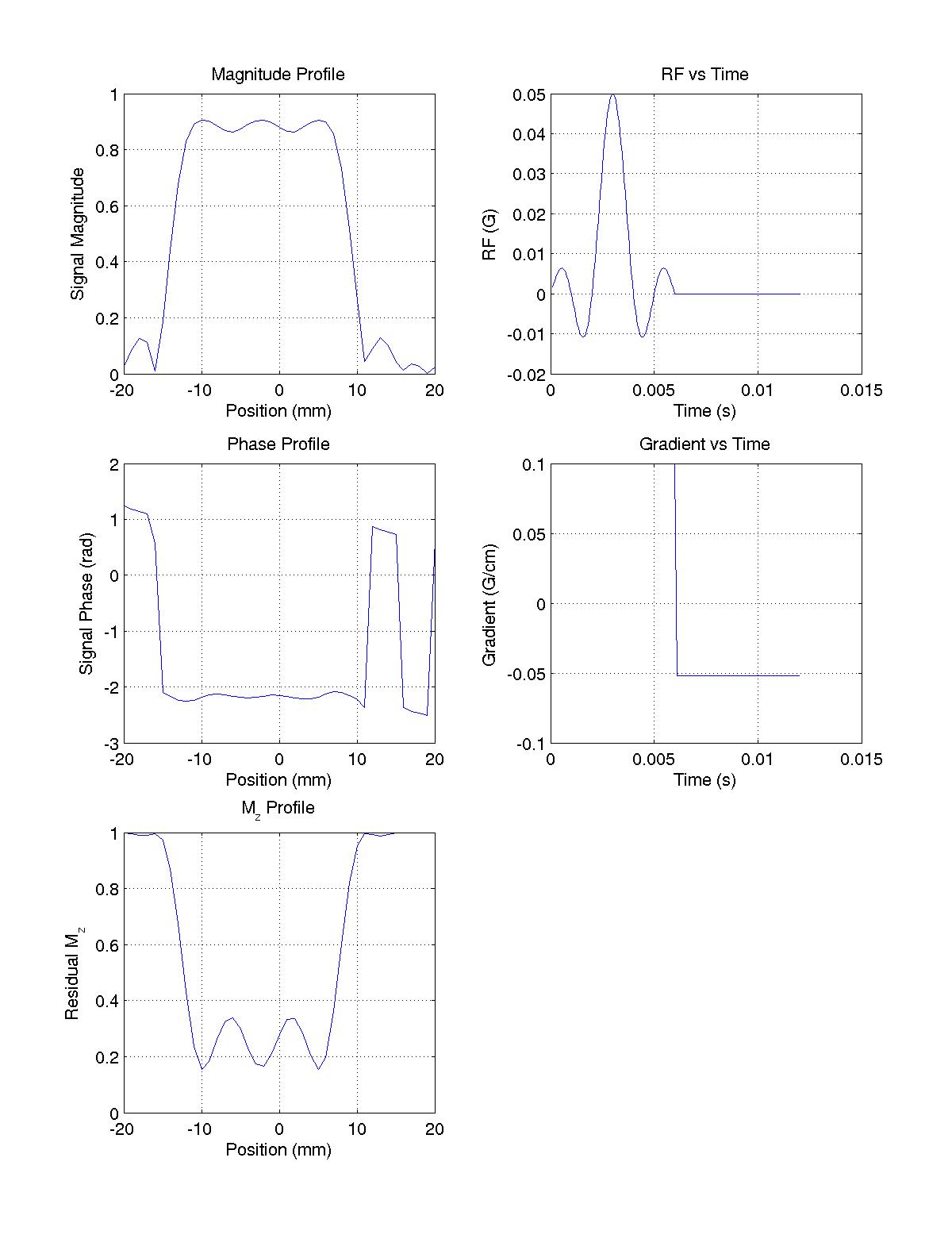
F-3d) Now modify the code of F-3c to shift the resonant frequency to 100 Hz (instead of 0 Hz). What happens to the slice profile?
Answer: The profile shifts by 2.3 mm. plot | Matlab Code
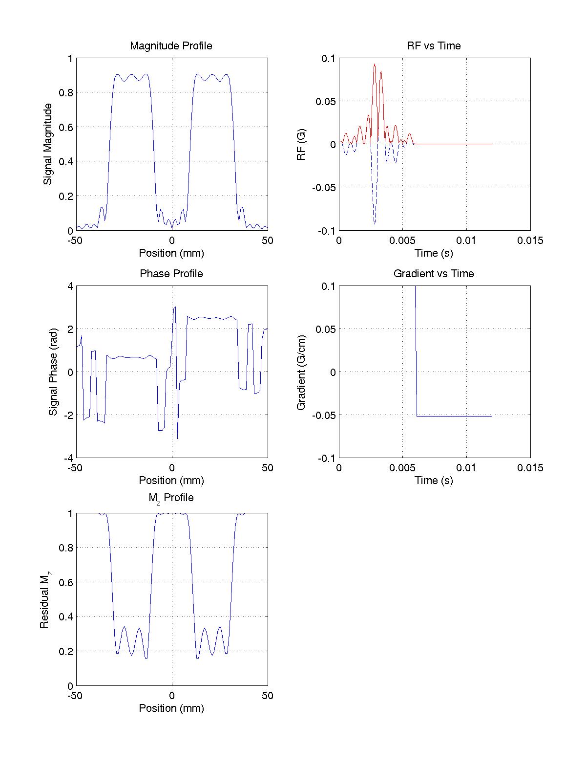
F-3e) Modulate the RF pulse in F-3c by a 900 Hz pure exponential, ie, exp(2*pi*900*i*t). Now plot the profile, RF and Gradient over the range [-50,50mm]. What happened?
Answer: plot | Matlab Code | The profile shifts by 1 cm. Changing the RF modulation frequency is how we excite slices off center. Notice that the phase of the profile changed.
F-3f) Now for fun, replace the RF with the RF of F-3e plus the RF modulated by a -900 Hz pure exponential and repeat. What does the answer tell you?
Answer: plot | Matlab Code | This answer should tell you that slice selction is almost linear. However, exciting two slices increased the peak RF, which is usally limited.
It should be apparent that the slice profile is related
to the Fourier transform of the RF. If we modulate the
RF by an exponential, we shift the slice profile. If
we modulate the RF by a cosine, we excite two slices.
F-4. Spectrally and Spatially Selective (2D) Excitation