All material on these pages is available free of charge for
teaching purposes.
Acknowledgment is appreciated where appropriate.
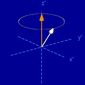
Precession
The resonance of nuclear magnetic resonance
is shown here. Nuclei in a magnetic field will precess around
the axis of the magnetic field, at the Larmor frequency,
which is proportional to the static field strength.
resonance.mpg
Relaxation and Precession
The component of magnetization parallel to the static
field will recover to its polarized state. This recovery
is exponential with a time constant called T1.
The component of magnetization perpendicular to the static
field will decay exponentially to zero, with a time constant
T2. This transvers magnetization is what precesses
about the field. The precession of transverse magnetization
induces the MR signal in the receive coil.
This animation shows T1 and T2 relaxation as well as precession.
T1 and T2 vary in biological tissue, and are the main sources
of image contrast in MRI.
relaxation.mpg
Excitation
An RF field, oriented in a transverse plane, alters the
net magnetic field. The magnetization will precess
about this net field. The RF field amplitude is much
smaller than the static field, so the net field is almost
unchanged. However, by rotating the RF field
direction (yellow arrow) at the Larmor frequency, magnetization
can be tipped arbitrarily into the transverse plane. The
resulting transverse magnetization gives an MR signal.
This animation shows the rotating Rf (B1) field, and the
path that the magnetization takes as it is excited into
the transverse plane.
nonrotb1tip.mpg
If a "rotating coordinate system" is used, we see that
we can arbitrarily tip magnetization about a transverse
axis.
rotb1tip.mpg
This series of animations shows the effect if the RF (B1)
is tuned to different frequencies. The numbers represent
the ratio of B1 frequency to Larmor frequency.
Note that at 1.0, B1 is tuned to the Larmor frequency,
and the magnetization is tipped a full 90 degrees.
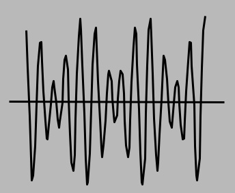
Here are shown two spins,
at different positions.
With a gradient on, the red spin precesses at a faster
frequency than the blue. (The red also has a higher
magnetization.) The following animation shows the
induced signals from the red and blue spins, and the
total signal.
signal.mpg
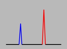
Although the total signal
seems unrecognizable, the
Fourier transform gives the two peaks corresponding
to the spin densities, here.
K-space
Any image can be written as a weighted sum of spatial harmonics.
Each point in k-space represents the weight that corresponds to
that harmonic. This movie shows the harmonics that correspond
to selected points in k-space.
The following show how the image forms as k-space is
filled in 3 common ways:
Static field inhomogeneities (and other effects) can result
in spins having different precession frequencies. A 180 degree
"refocosing" pulse can refocus the spins to a spin echo.
This animation shows the dephasing due to different frequencies,
and the refocusing effect of a 180 pulse.
spinecho.mpgSteady-State Imaging
These still to come!
Several different movies showing spins in steady
state, with and without alternating the RF are
available here. The most popular
is probably one showing multiple frequencies, and
alternating RF, here.
All code on these pages is available free of charge for
any use.
Acknowledgment is certainly appreciated where
appropriate.
I am very happy to discuss possible
applications and/or extensions of the information provided.